Discover SWOT L3 Unsmoothed data, and compare with CMEMS L4 SLA and IFREMER SST data

Tutorial Objectives

Download Swot data with cycle/passes numbers, using altimetry_downloader_aviso
Select data intersecting a geographical area, using altimetry.io
Download CMEMS map using copernicusmarine client, and plot Swot SLA with CMEMS SLA
Download SST map using copernicusmarine client and plot Swot SLA with SST

Note

Required environment to run this notebook:

xarray
numpy
matplotlib+cartopy+cmocean
altimetry_downloader_aviso: see documentation.
altimetry.io: available here.
copernicusmarine: see documentation.

Import + code

[1]:

import warnings
warnings.filterwarnings('ignore')

[2]:

# Configure logging if you want more details
import logging
logging.basicConfig(level=logging.INFO)

[3]:

from pathlib import Path
import xarray as xr
import numpy as np

import cartopy.crs as ccrs
import matplotlib.cm as mplcm
import matplotlib.pyplot as plt
import cmocean

import copernicusmarine

[4]:

def plot_datasets(datasets, variable, vminmax, title, extent=None):
    cb_args = dict(
        add_colorbar=True,
        cbar_kwargs={"shrink": 0.3}
    )

    plot_kwargs = dict(
        x="longitude",
        y="latitude",
        cmap="Spectral_r",
        vmin=vminmax[0],
        vmax=vminmax[1],
    )

    fig, ax = plt.subplots(figsize=(12, 8), subplot_kw=dict(projection=ccrs.PlateCarree()))
    if extent: ax.set_extent(extent)

    for ds in datasets:
        ds[variable].plot.pcolormesh(
            ax=ax,
            **plot_kwargs,
            **cb_args)
        cb_args=dict(add_colorbar=False)

    ax.set_title(title)
    ax.coastlines()
    gls = ax.gridlines(draw_labels=True)
    gls.top_labels=False
    gls.right_labels=False

    return ax

Parameters

Define a local filepath to download files

[5]:

output_dir= Path.home() / "TMP_DATA"

Define cycles and half_orbits numbers to download

Note

To look for Swot passes in a predefined geographical area and temporal period, use Search Swot tool.

[6]:

cycle_number = [2]
pass_number = [14, 169]

[7]:

# English channel
bbox = (-7, 46, 4, 52)
localbox = [-7, 4, 46, 52]

Download data using `altimetry_downloader_aviso`

[8]:

import altimetry_downloader_aviso as dl_aviso

[9]:

dl_aviso.get(
    'SWOT_L3_LR_SSH_Unsmoothed',
    output_dir=output_dir,
    cycle_number=cycle_number,
    pass_number=pass_number,
)

INFO:altimetry_downloader_aviso.catalog_client.client:Fetching products from Aviso's catalog...
INFO:altimetry_downloader_aviso.catalog_client.granule_discoverer:Filtering SWOT_L3_LR_SSH_Unsmoothed product with filters {'cycle_number': [2], 'pass_number': [14, 169]}...
INFO:altimetry_downloader_aviso.core:2 files to download. 0 files already exist.
INFO:altimetry_downloader_aviso.tds_client:File /home/atonneau/TMP_DATA/SWOT_L3_LR_SSH_Unsmoothed_002_014_20230811T132741_20230811T141908_v2.0.1.nc downloaded.
INFO:altimetry_downloader_aviso.tds_client:File /home/atonneau/TMP_DATA/SWOT_L3_LR_SSH_Unsmoothed_002_169_20230817T022159_20230817T031326_v2.0.1.nc downloaded.

[9]:

['/home/atonneau/TMP_DATA/SWOT_L3_LR_SSH_Unsmoothed_002_014_20230811T132741_20230811T141908_v2.0.1.nc',
 '/home/atonneau/TMP_DATA/SWOT_L3_LR_SSH_Unsmoothed_002_169_20230817T022159_20230817T031326_v2.0.1.nc']

Open data using `altimetry.io`

[8]:

from altimetry.io import AltimetryData, FileCollectionSource

Open data source

[9]:

alti_data = AltimetryData(
    source=FileCollectionSource(
        path=output_dir,
        ftype="SWOT_L3_LR_SSH",
        subset="Unsmoothed"
    ),
)

Query data

[10]:

ds_unsmoothed_14 = alti_data.query_orbit(
    cycle_number=cycle_number,
    pass_number=14,
    variables=['longitude', 'latitude', 'time', 'ssha_unfiltered', 'ssha_filtered', 'ssha_unedited', 'sigma0', 'quality_flag'],
    polygon=bbox
)

INFO:fcollections.implementations.optional._predicates:The bbox intersects with pass numbers (calval phase): [16]
INFO:fcollections.implementations.optional._predicates:The bbox intersects with pass numbers (science phase): [14, 42, 70, 85, 98, 113, 126, 141, 169, 197, 225, 264, 292, 320, 348, 363, 376, 391, 404, 419, 447, 475, 503, 542, 570]
INFO:fcollections.core._readers:Files to read: 1
INFO:fcollections.implementations.optional._area_selectors:Input longitudes does not fit in one of the known 360° intervals. Using [0, 360] (a copy of the input will be made)
INFO:fcollections.implementations.optional._area_selectors:Size of the dataset matching the bbox: {'num_lines': 3100, 'num_pixels': 519}

[11]:

ds_unsmoothed_169 = alti_data.query_orbit(
    cycle_number=cycle_number,
    pass_number=169,
    variables=['longitude', 'latitude', 'time', 'ssha_unfiltered', 'ssha_filtered', 'ssha_unedited', 'sigma0', 'quality_flag'],
    polygon=bbox
)

INFO:fcollections.implementations.optional._predicates:The bbox intersects with pass numbers (calval phase): [16]
INFO:fcollections.implementations.optional._predicates:The bbox intersects with pass numbers (science phase): [14, 42, 70, 85, 98, 113, 126, 141, 169, 197, 225, 264, 292, 320, 348, 363, 376, 391, 404, 419, 447, 475, 503, 542, 570]
INFO:fcollections.core._readers:Files to read: 1
INFO:fcollections.implementations.optional._area_selectors:Input longitudes does not fit in one of the known 360° intervals. Using [0, 360] (a copy of the input will be made)
INFO:fcollections.implementations.optional._area_selectors:Size of the dataset matching the bbox: {'num_lines': 3102, 'num_pixels': 519}

Visualise data

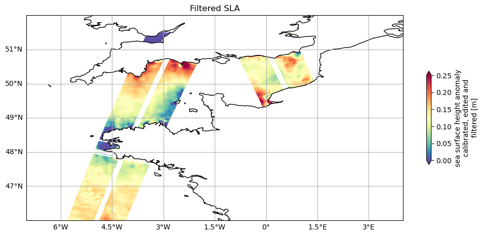
Let’s plot SLA for each cycle

[12]:

plot_datasets([ds_unsmoothed_169, ds_unsmoothed_14], 'ssha_filtered', (0, 0.25), 'Filtered SLA', extent=localbox)

[12]:

<GeoAxes: title={'center': 'Filtered SLA'}, xlabel='longitude (degrees East)\n[degrees_east]', ylabel='latitude (positive N, negative\nS) [degrees_north]'>

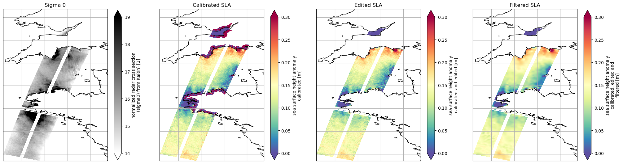
../_images/SWOT-Oceanography_ex_swot_l3_unsmoothed_27_1.png

Let’s plot SWOT KaRIn Sigma 0 and the different SLA available

[13]:

# Apply quality flag
ds_unsmoothed_169["sigma0"] = ds_unsmoothed_169.sigma0.where(ds_unsmoothed_169.quality_flag==0)
# Apply log 10
ds_unsmoothed_169["sigma0_log"] = 10*np.log10(ds_unsmoothed_169["sigma0"])

[14]:

localbox_zoom = [-5, -1.5, 46, 51]

[15]:

# set figure
fig, (ax1, ax2, ax3, ax4) = plt.subplots(1, 4, figsize=(25, 21), subplot_kw=dict(projection=ccrs.PlateCarree()))

plot_kwargs = dict(
    x="longitude",
    y="latitude",
    cmap="Spectral_r",
    vmin=0,
    vmax=0.3,
    cbar_kwargs={"shrink": 0.3}
)
plot_kwargs2 = dict(
    x="longitude",
    y="latitude",
    cmap="gray_r",
    vmin=14,
    vmax=19,
    cbar_kwargs={"shrink": 0.3}
)

ds_unsmoothed_169.sigma0_log.plot.pcolormesh(ax=ax1, **plot_kwargs2)
ax1.set_title("Sigma 0")

ds_unsmoothed_169.ssha_unedited.plot.pcolormesh(ax=ax2, **plot_kwargs)
ax2.set_title("Calibrated SLA")

ds_unsmoothed_169.ssha_unfiltered.plot.pcolormesh(ax=ax3, **plot_kwargs)
ax3.set_title("Edited SLA")

ds_unsmoothed_169.ssha_filtered.plot.pcolormesh(ax=ax4, **plot_kwargs)
ax4.set_title("Filtered SLA")

for ax in [ax1, ax2, ax3, ax4]:
    # ax.set_extent(localbox_zoom)
    ax.coastlines()
    ax.gridlines()

../_images/SWOT-Oceanography_ex_swot_l3_unsmoothed_31_0.png

Visualise SWOT SLA with L4 CMEMS SLA map

Download L4 CMEMS SLA maps with `copernicusmarine` client

[16]:

date_pass_14 = str(ds_unsmoothed_14.time.values[0].astype('datetime64[D]'))
date_pass_169 = str(ds_unsmoothed_169.time.values[0].astype('datetime64[D]'))

[17]:

# Load xarray dataset
duacs_l4 = copernicusmarine.open_dataset(
  dataset_id = "cmems_obs-sl_glo_phy-ssh_nrt_allsat-l4-duacs-0.25deg_P1D",
  start_datetime=date_pass_14,
  end_datetime=date_pass_169,
  minimum_longitude = bbox[0],
  maximum_longitude = bbox[2],
  minimum_latitude = bbox[1],
  maximum_latitude = bbox[3],
  variables = ['sla']
)

INFO - 2026-02-27T08:31:11Z - Selected dataset version: "202311"
INFO:copernicusmarine:Selected dataset version: "202311"
INFO - 2026-02-27T08:31:11Z - Selected dataset part: "default"
INFO:copernicusmarine:Selected dataset part: "default"

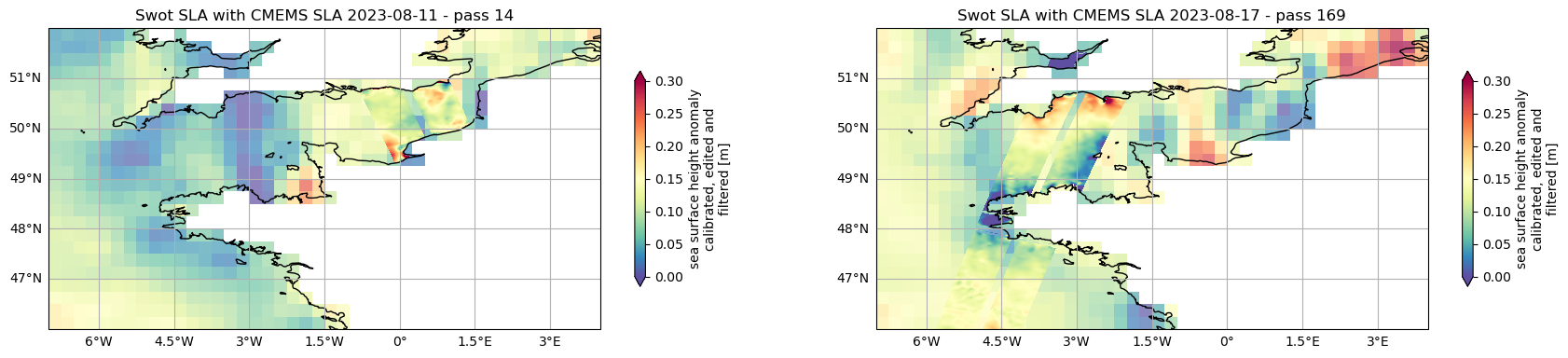
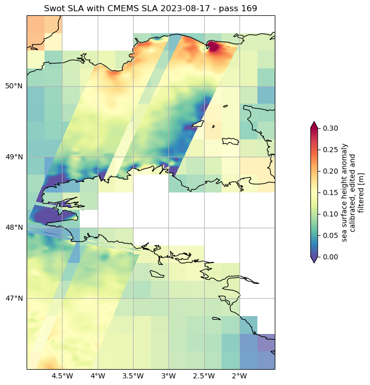
Visualise SWOT SLA with CMEMS SLA

[18]:

localbox_zoom2 = [-5, -1.5, 46, 51]

[19]:

plot_kwargs = dict(
    x="longitude",
    y="latitude",
    cmap="Spectral_r",
    vmin=0,
    vmax=0.3
)
fig, (ax1, ax2) = plt.subplots(1, 2, figsize=(21, 15), subplot_kw=dict(projection=ccrs.PlateCarree()))

duacs_l4.sla.sel(time=np.datetime64(date_pass_14), method='nearest').plot.pcolormesh(
    ax=ax1,
    alpha=0.7,
    add_colorbar=False,
    **plot_kwargs)
ds_unsmoothed_14['ssha_filtered'].plot.pcolormesh(
    ax=ax1,
    cbar_kwargs={"shrink": 0.2},
    **plot_kwargs)
ax1.set_title(f'Swot SLA with CMEMS SLA {date_pass_14} - pass 14')
ax1.set_extent(localbox)

duacs_l4.sla.sel(time=np.datetime64(date_pass_169), method='nearest').plot.pcolormesh(
    ax=ax2,
    alpha=0.7,
    add_colorbar=False,
    **plot_kwargs)
ds_unsmoothed_169['ssha_filtered'].plot.pcolormesh(
    ax=ax2,
    cbar_kwargs={"shrink": 0.2},
    **plot_kwargs)
ax2.set_title(f'Swot SLA with CMEMS SLA {date_pass_169} - pass 169')
ax2.set_extent(localbox)

for ax in [ax1, ax2]:
    ax.coastlines()
    gls = ax.gridlines(draw_labels=True)
    gls.top_labels=False
    gls.right_labels=False

../_images/SWOT-Oceanography_ex_swot_l3_unsmoothed_38_0.png

[20]:

fig, ax = plt.subplots(figsize=(18, 9), subplot_kw=dict(projection=ccrs.PlateCarree()))

duacs_l4.sla.sel(time=np.datetime64(date_pass_169), method='nearest').plot.pcolormesh(
    ax=ax,
    alpha=0.7,
    add_colorbar=False,
    **plot_kwargs)
ds_unsmoothed_169['ssha_filtered'].plot.pcolormesh(
    ax=ax,
    cbar_kwargs={"shrink": 0.4},
    **plot_kwargs)
ax.set_title(f'Swot SLA with CMEMS SLA {date_pass_169} - pass 169')
ax.set_extent(localbox_zoom2)
ax.coastlines()
gls = ax.gridlines(draw_labels=True)
gls.top_labels=False
gls.right_labels=False

../_images/SWOT-Oceanography_ex_swot_l3_unsmoothed_39_0.png

Visualise SWOT SLA with IFREMER SST map

Download SST maps with `copernicusmarine` client

[21]:

# Load xarray dataset
sst = copernicusmarine.open_dataset(
  dataset_id = "IFREMER-GLOB-SST-L3-NRT-OBS_FULL_TIME_SERIE",
  start_datetime=date_pass_14,
  end_datetime=date_pass_169,
  minimum_longitude = bbox[0],
  maximum_longitude = bbox[2],
  minimum_latitude = bbox[1],
  maximum_latitude = bbox[3],
  variables = ['sea_surface_temperature']
)

INFO - 2026-02-27T08:34:40Z - Selected dataset version: "202211"
INFO:copernicusmarine:Selected dataset version: "202211"
INFO - 2026-02-27T08:34:40Z - Selected dataset part: "default"
INFO:copernicusmarine:Selected dataset part: "default"

[22]:

ds_sst = sst.sel(time=np.datetime64(date_pass_169), method='nearest')

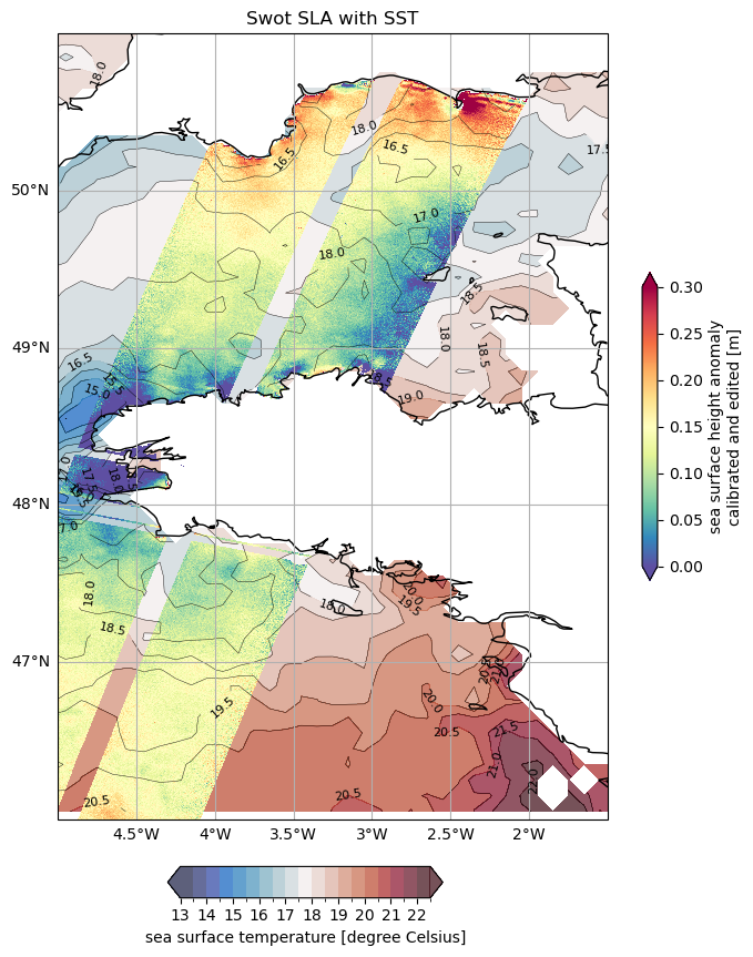
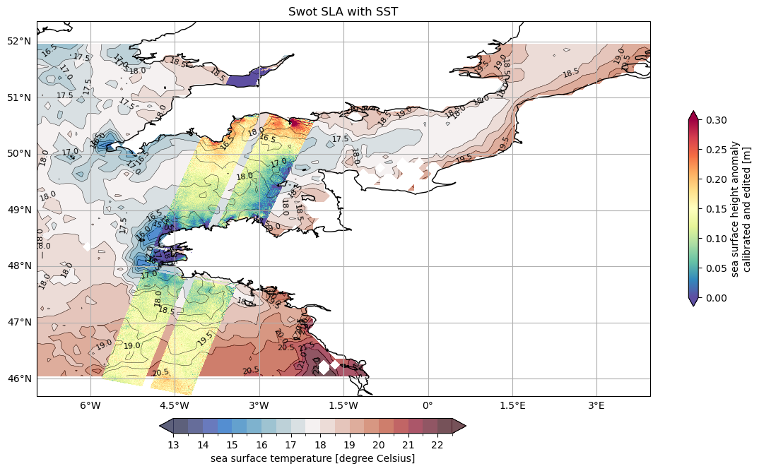
Visualise SWOT SLA with SST

[23]:

fig, ax = plt.subplots(figsize=(14, 12), subplot_kw=dict(projection=ccrs.PlateCarree()))

plot_kwargs = dict(
    x="longitude",
    y="latitude",
    cmap="Spectral_r"
)

cb_args = dict(
    add_colorbar=True,
    cbar_kwargs={"shrink": 0.3}
)

cmap_sst = cmocean.cm.balance
levs_sst = np.arange(13,23,step=0.5)
norm_sst = mplcm.colors.BoundaryNorm(levs_sst,cmap_sst.N)

contourf = ax.contourf(ds_sst.longitude,
                      ds_sst.latitude,
                      ds_sst.sea_surface_temperature-273.15,
                      levs_sst,
                      cmap=cmap_sst,
                      norm=norm_sst,
                      alpha=0.7,
                      extend='both')

contour = ax.contour(ds_sst.longitude,
                      ds_sst.latitude,
                      ds_sst.sea_surface_temperature-273.15,
                      levels=levs_sst,
                      colors="black",
                      linewidths=0.3)

ax.clabel(contour, inline=1, fontsize=8)

cax = ax.inset_axes([0.2, -0.1, 0.5, 0.04])

cb_sst = plt.colorbar(contourf, cax=cax, orientation='horizontal', pad=0.005, shrink=0.5)
cb_sst.set_label('sea surface temperature [degree Celsius]')
cb_sst.ax.tick_params(labelsize=10)

ds_unsmoothed_169['ssha_unfiltered'].plot.pcolormesh(
    ax=ax,
    vmin=0,
    vmax=0.3,
    **plot_kwargs,
    **cb_args)

ax.coastlines()
gls = ax.gridlines(draw_labels=True)
gls.top_labels=False
gls.right_labels=False
ax.set_title('Swot SLA with SST')

[23]:

Text(0.5, 1.0, 'Swot SLA with SST')

../_images/SWOT-Oceanography_ex_swot_l3_unsmoothed_45_1.png

[24]:

fig, ax = plt.subplots(figsize=(14, 12), subplot_kw=dict(projection=ccrs.PlateCarree()))

contourf = ax.contourf(ds_sst.longitude,
                      ds_sst.latitude,
                      ds_sst.sea_surface_temperature-273.15,
                      levs_sst,
                      cmap=cmap_sst,
                      norm=norm_sst,
                      alpha=0.7,
                      extend='both')

contour = ax.contour(ds_sst.longitude,
                      ds_sst.latitude,
                      ds_sst.sea_surface_temperature-273.15,
                      levels=levs_sst,
                      colors="black",
                      linewidths=0.3)

ax.clabel(contour, inline=1, fontsize=8)

cax = ax.inset_axes([0.2, -0.1, 0.5, 0.04])

cb_sst = plt.colorbar(contourf, cax=cax, orientation='horizontal', pad=0.005, shrink=0.5)
cb_sst.set_label('sea surface temperature [degree Celsius]')
cb_sst.ax.tick_params(labelsize=10)

ds_unsmoothed_169['ssha_unfiltered'].plot.pcolormesh(
    ax=ax,
    vmin=0,
    vmax=0.3,
    **plot_kwargs,
    **cb_args)

ax.coastlines()
gls = ax.gridlines(draw_labels=True)
gls.top_labels=False
gls.right_labels=False
ax.set_title('Swot SLA with SST')
fig.set_figwidth(8)
ax.set_extent(localbox_zoom2)

../_images/SWOT-Oceanography_ex_swot_l3_unsmoothed_46_0.png

Download notebook.