SWOT L3 KaRIn Wind Wave Data Products
The SWOT KaRIn Level-3 Wind Wave product (L3_LR_WIND_WAVE) is an innovative product derived from the Unsmoothed L3_LR_SSH product based on the algorithm presented in Ardhuin et al., 2024. It takes advantage of the KaRIn Low Rate (LR) chain’s ability to resolve waves larger than about 500 meters in wavelength (about 18 s) and provides detailed information on the characteristics of these wave regimes, including significant wave height (SWH), dominant wavelength, and wave propagation direction. These regimes are typically associated with long-period swells and extreme events that play a critical role in ocean dynamics, coastal processes, and maritime operations.
SWOT L3_LR_WIND_WAVE product is organized in 2 subproducts:
Light L3_LR_WIND_WAVE (or lightweight), which includes the spectrum of KaRIn L3 250-m SSHA corrected from instrumental effects, expressed in both cartesian and polar coordinates, the swell partition of the spectrum and the wave parameters integrated over this partition for both WW3 model and KaRIn (significant wave height, wavelength and direction)
Extended L3_LR_WIND_WAVE, which includes the same variables as the light product below plus the WW3 spectrum in the same frequency grid as the KaRIn spectrum, the KaRIn transfer functions used for correction and some parameters derived from KaRIn observations (coherence, mean backscatter…)
Data can be explored at Swot LR L3 Wind Wave catalog.
For more information about this product, please consult its User handbook.
Tutorial Objectives
Download files using
altimetry_downloader_avisoOpen data using
altimetry.ioPresent SWOT L3 Wind Wave data products (light and extended products)
Plot integrated wave parameters
Plot wave direction
Plot KaRIn Wave Spectrum
Note
Required environment to run this notebook:
xarray+numpymatplotlib+cartopy+cmoceangeopandas+shapelypyinterp+dask+numbaaltimetry_downloader_aviso: see documentation.altimetry.io: available here.
Imports + code
# Configure logging if you want more details
import logging
logging.basicConfig(level=logging.INFO)
from pathlib import Path
import xarray as xr
import numpy as np

import cartopy.crs as ccrs
import cartopy.feature as cfeature
from matplotlib import colors
import matplotlib.pyplot as plt
def custom_ax(ax, crs=ccrs.PlateCarree(central_longitude=0), extent=None):
    ax.coastlines(resolution='50m')
    gl = ax.gridlines(
        crs=crs,
        draw_labels=True,
        linewidth=1,
        color='gray',
        alpha=0.8
    )
    gl.top_labels = gl.right_labels = False
    if extent:
        ax.set_extent(
            extent,
            crs=crs
        )
    return ax
def get_mask_border(mask, fx1d, fy1d):
    import shapely.geometry
    import shapely.ops

    dfx = fx1d[1] - fx1d[0]
    dfy = fy1d[1] - fy1d[0]
    xbound = np.append(fx1d - dfx/2, fx1d[-1] + dfx/2)
    ybound = np.append(fy1d - dfy/2, fy1d[-1] + dfy/2)
    geoms = []
    for yidx, xidx in zip(*np.where(mask)):
        geoms.append(shapely.geometry.box(xbound[xidx], ybound[yidx], xbound[xidx+1], ybound[yidx+1]))
    full_geom = shapely.ops.unary_union(geoms)
    x,y = full_geom.exterior.xy
    return np.asarray(x), np.asarray(y)

def rotate_angle_from_NE_to_SWOT_ref_system(angle, track_angle):
    angle_swot = angle - track_angle
    angle_swot = (angle_swot + 180)%360 - 180
    return angle_swot
Parameters
Define a local filepath to download files
output_dir= Path.home() / "TMP_DATA"
Define cycles and half_orbits numbers to download
cycle_number = 6
pass_number = 567
Download data using altimetry_downloader_aviso
import altimetry_downloader_aviso as dl_aviso
downloaded_files = dl_aviso.get(
    'SWOT_L3_LR_WIND_WAVE_Light',
    output_dir=output_dir,
    cycle_number=cycle_number,
    pass_number=pass_number,
)
downloaded_files
INFO:altimetry_downloader_aviso.catalog_client.client:Fetching products from Aviso's catalog...
INFO:altimetry_downloader_aviso.catalog_client.granule_discoverer:Filtering SWOT_L3_LR_WIND_WAVE_Light product with filters {'cycle_number': 6, 'pass_number': 567}...
INFO:altimetry_downloader_aviso.core:1 files to download. 0 files already exist.
INFO:altimetry_downloader_aviso.tds_client:File /home/atonneau/TMP_DATA/SWOT_L3_LR_WIND_WAVE_006_567_20231122T183814_20231122T192938_v2.0.nc downloaded.
['/home/atonneau/TMP_DATA/SWOT_L3_LR_WIND_WAVE_006_567_20231122T183814_20231122T192938_v2.0.nc']
downloaded_files = dl_aviso.get(
    'SWOT_L3_LR_WIND_WAVE_Extended',
    output_dir=output_dir,
    cycle_number=cycle_number,
    pass_number=pass_number,
)
downloaded_files
INFO:altimetry_downloader_aviso.catalog_client.client:Fetching products from Aviso's catalog...
INFO:altimetry_downloader_aviso.catalog_client.granule_discoverer:Filtering SWOT_L3_LR_WIND_WAVE_Extended product with filters {'cycle_number': 6, 'pass_number': 567}...
INFO:altimetry_downloader_aviso.core:1 files to download. 0 files already exist.
INFO:altimetry_downloader_aviso.tds_client:File /home/atonneau/TMP_DATA/SWOT_L3_LR_WIND_WAVE_Extended_006_567_20231122T183814_20231122T192938_v2.0.nc downloaded.
['/home/atonneau/TMP_DATA/SWOT_L3_LR_WIND_WAVE_Extended_006_567_20231122T183814_20231122T192938_v2.0.nc']
downloaded_files = dl_aviso.get(
    'SWOT_L3_LR_SSH_Unsmoothed',
    output_dir=output_dir,
    cycle_number=cycle_number,
    pass_number=pass_number,
)
downloaded_files
INFO:altimetry_downloader_aviso.catalog_client.client:Fetching products from Aviso's catalog...
INFO:altimetry_downloader_aviso.catalog_client.granule_discoverer:Filtering SWOT_L3_LR_SSH_Unsmoothed product with filters {'cycle_number': 6, 'pass_number': 567}...
INFO:altimetry_downloader_aviso.core:1 files to download. 0 files already exist.
INFO:altimetry_downloader_aviso.tds_client:File /home/atonneau/TMP_DATA/SWOT_L3_LR_SSH_Unsmoothed_006_567_20231122T183813_20231122T192940_v2.0.1.nc downloaded.
['/home/atonneau/TMP_DATA/SWOT_L3_LR_SSH_Unsmoothed_006_567_20231122T183813_20231122T192940_v2.0.1.nc']
Discover the product
Light product
The main geophysical quantity contained in the L3 Wind Wave product is the “wave” spectrum. This wave spectrum is computed as the power spectral density (PSD) of the KaRIn heights (sea surface heights anomalies or SSHA).
In the Light product, the spectrum is estimated over a “box” of SSHA of 40x40 km by using a Welch (1967) approach : the box is sub-divided in tiles -of 5 km size and overlaping by 50 % of their surface in this case- and a fast fourier transform (FFT) is computed over each tile. Finally, the transforms obtained for the same box are averaged together.
As explained in the User handbook (sections 2.4 and 2.5), the product provides also an identification of the wave partition of the spectrum (aka “swell mask”) as well as the respective wave integrated parameters significant wave height (𝐻18), wavelength (𝐿18) and direction (ϕ_18).
To sum up, the Light product contains:
KaRIn-based wave spectrum, derived from KaRIn SSHA, computed using 40km boxes and 5km tiles
a swell mask
the respective wave integrated parameters
Additionally, the Light product provides:
wave spectrum from model (WW3) for the same location as KaRIn-based spectrum
the respective wave model integrated parameters
Light product content
Open data using cnes_alti_reader
from altimetry.io import AltimetryData, FileCollectionSource
alti_data = AltimetryData(
    source=FileCollectionSource(
        path=output_dir,
        ftype="SWOT_L3_LR_WIND_WAVE",
        subset="Light"
    ),
)
ds_light = alti_data.query_orbit(
    cycle_number=cycle_number,
    pass_number=pass_number
)
INFO:fcollections.core._readers:Files to read: 1
ds_light
<xarray.Dataset> Size: 13MB
Dimensions:              (n_box: 986, nfy: 21, nfx: 20, nf: 11, nphi: 72)
Coordinates:
    longitude            (n_box) float64 8kB dask.array<chunksize=(986,), meta=np.ndarray>
    latitude             (n_box) float64 8kB dask.array<chunksize=(986,), meta=np.ndarray>
Dimensions without coordinates: n_box, nfy, nfx, nf, nphi
Data variables: (12/22)
    track_angle          (n_box) float64 8kB dask.array<chunksize=(986,), meta=np.ndarray>
    L18                  (n_box) float64 8kB dask.array<chunksize=(986,), meta=np.ndarray>
    H18_model            (n_box) float64 8kB dask.array<chunksize=(986,), meta=np.ndarray>
    swell_mask           (n_box, nfy, nfx) float64 3MB dask.array<chunksize=(986, 21, 20), meta=np.ndarray>
    E_f_phi_SWOT_masked  (n_box, nf, nphi) float64 6MB dask.array<chunksize=(986, 11, 72), meta=np.ndarray>
    phi_vector           (nphi) float64 576B dask.array<chunksize=(72,), meta=np.ndarray>
    ...                   ...
    quality_flag         (n_box) float64 8kB dask.array<chunksize=(986,), meta=np.ndarray>
    longitude_model      (n_box) float64 8kB dask.array<chunksize=(986,), meta=np.ndarray>
    time                 (n_box) datetime64[ns] 8kB dask.array<chunksize=(986,), meta=np.ndarray>
    time_model           (n_box) datetime64[ns] 8kB dask.array<chunksize=(986,), meta=np.ndarray>
    phi18_model          (n_box) float64 8kB dask.array<chunksize=(986,), meta=np.ndarray>
    Efxfy_SWOT           (n_box, nfy, nfx) float64 3MB dask.array<chunksize=(986, 21, 20), meta=np.ndarray>
Attributes: (12/32)
    Conventions:           CF-1.7
    Metadata_Conventions:  Unidata Dataset Discovery v1.0
    cdm_data_type:         Swath
    comment:               Wind/wave measured by KaRIn
    contact:               aviso@altimetry.fr
    creator_email:         aviso@altimetry.fr
    ...                    ...
    time_coverage_start:   2023-11-22T18:38:14Z
    time_coverage_end:     2023-11-22T19:29:38Z
    title:                 SWOT KaRIn Global Ocean swath Wind Wave L3 product
    NCO:                   netCDF Operators version 5.0.1 (Homepage = http://...
    project:               VAGUES, DESMOS, DUACS
history: Mon Feb 24 13:40:38 2025: ncatted -O -a platform,g...Extended product
The Extended product explores additional combinations of box and tile sizes
The tile size determines the dimensions (number of frequencies) of the spectrum. While Light files have a classic NetCDF structure, Extended files use a group and subgroup indexing approach. Each group corresponds to a specific tile size (in km). Within each tile group, there is a different subgroup per box size (in km).
The structure of the Extended product is as follows:
40 km boxes with 10 km tiles
20 km boxes with 10 km tiles
10 km boxes with 5 km tiles:
The Extended product contains the same variables as the Light product plus additional ones useful for users desiring to have a deeper insight on the KaRIn measurement, namely:
Approximate KaRIn transfer functions
Phase of the cross-spectrum between SSH and NRCS (useful for removing 180° wave propagation ambiguity)
Coherence of SSH and NRCS spectra
Real part of SSH-NRCS cross-spectrum
Extended product content
Extended Netcdf file structure:
Group |
Dimensions |
Subgroup |
Dimensions |
|---|---|---|---|
tile_5km |
nfy = 21 ; nfx = 20 ; nphi = 72 ; nf = 11 ; |
box_40km |
n_box = 986 ; nind = 4 ; |
box_10km |
n_box = 27650 ; nind = 4 ; |
||
tile_10km |
nfy = 42 ; nfx = 40 ; nphi = 144 ; nf = 20 ; |
box_20km |
n_box = 5922 ; nind = 4 ; |
box_40km |
n_box = 986 ; nind = 4 ; |
Choose the combination of tile-box
alti_data = AltimetryData(
    source=FileCollectionSource(
        path=output_dir,
        ftype="SWOT_L3_LR_WIND_WAVE",
        subset="Extended"
    ),
)
ds_box = alti_data.query_orbit(
    cycle_number=cycle_number,
    pass_number=pass_number,
    backend_kwargs={"tile":10, "box":20}
)
ds_box
INFO:fcollections.core._readers:Files to read: 1
INFO:fcollections.core._readers:Files to read: 1
<xarray.Dataset> Size: 615MB
Dimensions:              (nfy: 42, nfx: 40, nphi: 144, nf: 20, n_box: 5922,
                          nind: 4)
Coordinates:
    longitude            (n_box) float64 47kB dask.array<chunksize=(5922,), meta=np.ndarray>
    latitude             (n_box) float64 47kB dask.array<chunksize=(5922,), meta=np.ndarray>
Dimensions without coordinates: nfy, nfx, nphi, nf, n_box, nind
Data variables: (12/33)
    filter_PTR           (nfy, nfx) float64 13kB dask.array<chunksize=(42, 40), meta=np.ndarray>
    phi_vector           (nphi) float64 1kB dask.array<chunksize=(144,), meta=np.ndarray>
    fx2D                 (nfy, nfx) float64 13kB dask.array<chunksize=(42, 40), meta=np.ndarray>
    f_vector             (nf) float64 160B dask.array<chunksize=(20,), meta=np.ndarray>
    fy2D                 (nfy, nfx) float64 13kB dask.array<chunksize=(42, 40), meta=np.ndarray>
    filter_OBP           (nfy, nfx) float64 13kB dask.array<chunksize=(42, 40), meta=np.ndarray>
    ...                   ...
    longitude_model      (n_box) float64 47kB dask.array<chunksize=(5922,), meta=np.ndarray>
    time                 (n_box) datetime64[ns] 47kB dask.array<chunksize=(5922,), meta=np.ndarray>
    time_model           (n_box) datetime64[ns] 47kB dask.array<chunksize=(5922,), meta=np.ndarray>
    phi18_model          (n_box) float64 47kB dask.array<chunksize=(5922,), meta=np.ndarray>
    Hs_model             (n_box) float64 47kB dask.array<chunksize=(5922,), meta=np.ndarray>
Efxfy_SWOT (n_box, nfy, nfx) float64 80MB dask.array<chunksize=(2961, 21, 20), meta=np.ndarray>ds_box['longitude'] = (ds_box['longitude'] + 180)%360 - 180
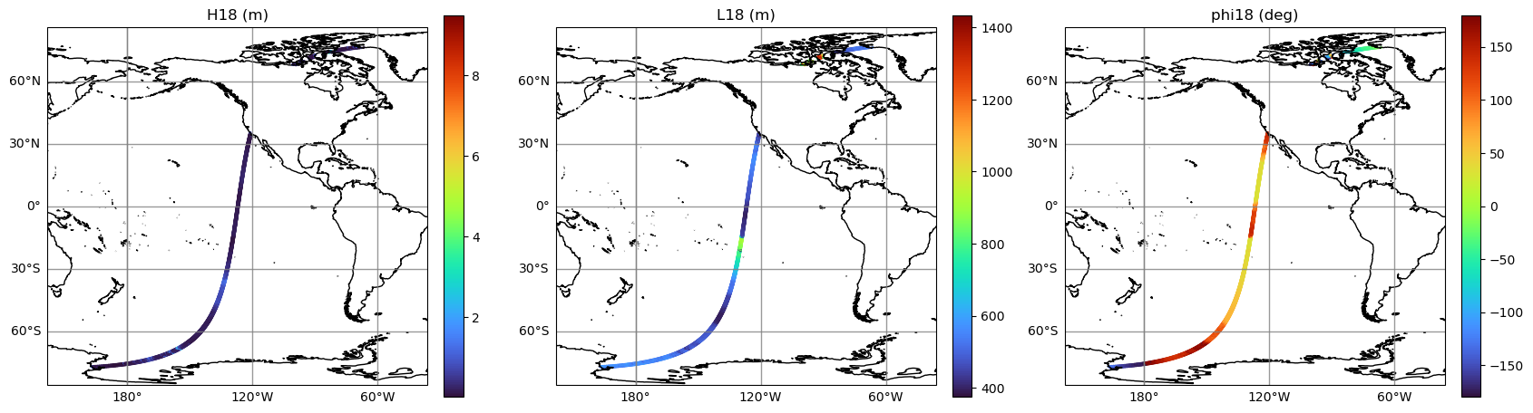
Plot map of integrated wave parameters
Parameter |
Description |
Unit |
|---|---|---|
𝐻18 |
Significant wave height for waves longer than 18s |
meter |
𝐿18 |
Wavelength taken as the ratio of zeroth and first moment of the spectrum (m0/m1) |
meter |
ϕ_18 |
Swell propagation direction taken as the direction of the mean wavenumber vector |
degree |
integrated_wparams = ['H18', 'L18', 'phi18']
integrated_wparams_titles = ['H18 (m)', 'L18 (m)', 'phi18 (deg)']
central_lon = ds_box['longitude'].values[ds_box.sizes['n_box']//2]

f, axs = plt.subplots(
    1,
    len(integrated_wparams),
    figsize=(17,7),
    sharex=True,
    sharey=True,
    subplot_kw={'projection':ccrs.PlateCarree(central_longitude=central_lon)}
)

for i, v in enumerate(integrated_wparams):
    ax = axs[i]
    ax = custom_ax(ax)

    im = ax.scatter(
        ds_box.longitude,
        ds_box.latitude,
        c= ds_box[v],
        s=1,
        cmap='turbo',
        transform=ccrs.PlateCarree()
    )
    cbar = plt.colorbar(im, ax=ax, fraction=0.046, pad=0.04)
    ax.set_title(integrated_wparams_titles[i])

plt.tight_layout()
plt.show()
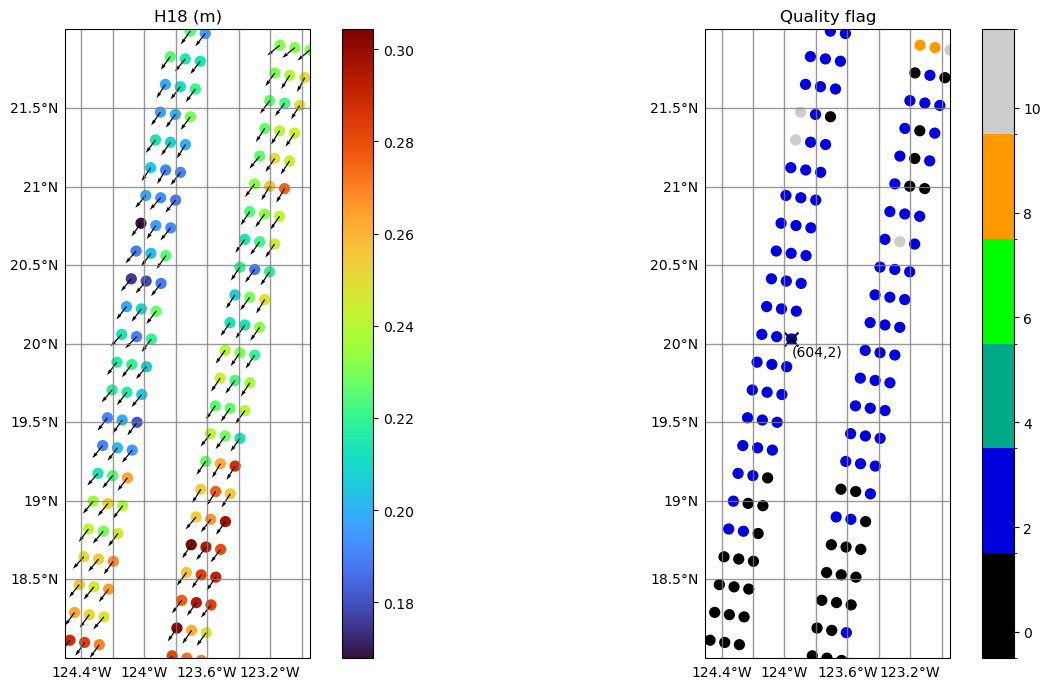
Zoom into specific region: show 𝐻18, wave direction with arrows and quality flag
Show 𝐻18 with wave direction
Show quality flag
Select arbitrary point and show box indices
Geographical parameters
Subset data with latitude range
ds_sel = alti_data.query_orbit(
    cycle_number=cycle_number,
    pass_number=pass_number,
    backend_kwargs={"tile":10, "box":20},
    polygon=(-180, 17.9, 180, 22)
)
ds_sel
INFO:fcollections.implementations.optional._predicates:The bbox intersects with pass numbers (calval phase): [1, 2, 3, 4, 5, 6, 7, 8, 9, 10, 11, 12, 13, 14, 15, 16, 17, 18, 19, 20, 21, 22, 23, 24, 25, 26, 27, 28]
INFO:fcollections.implementations.optional._predicates:The bbox intersects with pass numbers (science phase): [1, 2, 3, 4, 5, 6, 7, 8, 9, 10, 11, 12, 13, 14, 15, 16, 17, 18, 19, 20, 21, 22, 23, 24, 25, 26, 27, 28, 29, 30, 31, 32, 33, 34, 35, 36, 37, 38, 39, 40, 41, 42, 43, 44, 45, 46, 47, 48, 49, 50, 51, 52, 53, 54, 55, 56, 57, 58, 59, 60, 61, 62, 63, 64, 65, 66, 67, 68, 69, 70, 71, 72, 73, 74, 75, 76, 77, 78, 79, 80, 81, 82, 83, 84, 85, 86, 87, 88, 89, 90, 91, 92, 93, 94, 95, 96, 97, 98, 99, 100, 101, 102, 103, 104, 105, 106, 107, 108, 109, 110, 111, 112, 113, 114, 115, 116, 117, 118, 119, 120, 121, 122, 123, 124, 125, 126, 127, 128, 129, 130, 131, 132, 133, 134, 135, 136, 137, 138, 139, 140, 141, 142, 143, 144, 145, 146, 147, 148, 149, 150, 151, 152, 153, 154, 155, 156, 157, 158, 159, 160, 161, 162, 163, 164, 165, 166, 167, 168, 169, 170, 171, 172, 173, 174, 175, 176, 177, 178, 179, 180, 181, 182, 183, 184, 185, 186, 187, 188, 189, 190, 191, 192, 193, 194, 195, 196, 197, 198, 199, 200, 201, 202, 203, 204, 205, 206, 207, 208, 209, 210, 211, 212, 213, 214, 215, 216, 217, 218, 219, 220, 221, 222, 223, 224, 225, 226, 227, 228, 229, 230, 231, 232, 233, 234, 235, 236, 237, 238, 239, 240, 241, 242, 243, 244, 245, 246, 247, 248, 249, 250, 251, 252, 253, 254, 255, 256, 257, 258, 259, 260, 261, 262, 263, 264, 265, 266, 267, 268, 269, 270, 271, 272, 273, 274, 275, 276, 277, 278, 279, 280, 281, 282, 283, 284, 285, 286, 287, 288, 289, 290, 291, 292, 293, 294, 295, 296, 297, 298, 299, 300, 301, 302, 303, 304, 305, 306, 307, 308, 309, 310, 311, 312, 313, 314, 315, 316, 317, 318, 319, 320, 321, 322, 323, 324, 325, 326, 327, 328, 329, 330, 331, 332, 333, 334, 335, 336, 337, 338, 339, 340, 341, 342, 343, 344, 345, 346, 347, 348, 349, 350, 351, 352, 353, 354, 355, 356, 357, 358, 359, 360, 361, 362, 363, 364, 365, 366, 367, 368, 369, 370, 371, 372, 373, 374, 375, 376, 377, 378, 379, 380, 381, 382, 383, 384, 385, 386, 387, 388, 389, 390, 391, 392, 393, 394, 395, 396, 397, 398, 399, 400, 401, 402, 403, 404, 405, 406, 407, 408, 409, 410, 411, 412, 413, 414, 415, 416, 417, 418, 419, 420, 421, 422, 423, 424, 425, 426, 427, 428, 429, 430, 431, 432, 433, 434, 435, 436, 437, 438, 439, 440, 441, 442, 443, 444, 445, 446, 447, 448, 449, 450, 451, 452, 453, 454, 455, 456, 457, 458, 459, 460, 461, 462, 463, 464, 465, 466, 467, 468, 469, 470, 471, 472, 473, 474, 475, 476, 477, 478, 479, 480, 481, 482, 483, 484, 485, 486, 487, 488, 489, 490, 491, 492, 493, 494, 495, 496, 497, 498, 499, 500, 501, 502, 503, 504, 505, 506, 507, 508, 509, 510, 511, 512, 513, 514, 515, 516, 517, 518, 519, 520, 521, 522, 523, 524, 525, 526, 527, 528, 529, 530, 531, 532, 533, 534, 535, 536, 537, 538, 539, 540, 541, 542, 543, 544, 545, 546, 547, 548, 549, 550, 551, 552, 553, 554, 555, 556, 557, 558, 559, 560, 561, 562, 563, 564, 565, 566, 567, 568, 569, 570, 571, 572, 573, 574, 575, 576, 577, 578, 579, 580, 581, 582, 583, 584]
INFO:fcollections.core._readers:Files to read: 1
INFO:fcollections.core._readers:Files to read: 1
INFO:fcollections.implementations.optional._area_selectors:Size of the dataset matching the bbox: {'n_box': 140, 'nfy': 42, 'nfx': 40, 'nf': 20, 'nphi': 144, 'nind': 4}
<xarray.Dataset> Size: 15MB
Dimensions:              (nfy: 42, nfx: 40, nphi: 144, nf: 20, n_box: 140,
                          nind: 4)
Coordinates:
    longitude            (n_box) float64 1kB dask.array<chunksize=(140,), meta=np.ndarray>
    latitude             (n_box) float64 1kB dask.array<chunksize=(140,), meta=np.ndarray>
Dimensions without coordinates: nfy, nfx, nphi, nf, n_box, nind
Data variables: (12/33)
    filter_PTR           (nfy, nfx) float64 13kB dask.array<chunksize=(42, 40), meta=np.ndarray>
    phi_vector           (nphi) float64 1kB dask.array<chunksize=(144,), meta=np.ndarray>
    fx2D                 (nfy, nfx) float64 13kB dask.array<chunksize=(42, 40), meta=np.ndarray>
    f_vector             (nf) float64 160B dask.array<chunksize=(20,), meta=np.ndarray>
    fy2D                 (nfy, nfx) float64 13kB dask.array<chunksize=(42, 40), meta=np.ndarray>
    filter_OBP           (nfy, nfx) float64 13kB dask.array<chunksize=(42, 40), meta=np.ndarray>
    ...                   ...
    longitude_model      (n_box) float64 1kB dask.array<chunksize=(140,), meta=np.ndarray>
    time                 (n_box) datetime64[ns] 1kB dask.array<chunksize=(140,), meta=np.ndarray>
    time_model           (n_box) datetime64[ns] 1kB dask.array<chunksize=(140,), meta=np.ndarray>
    phi18_model          (n_box) float64 1kB dask.array<chunksize=(140,), meta=np.ndarray>
    Hs_model             (n_box) float64 1kB dask.array<chunksize=(140,), meta=np.ndarray>
Efxfy_SWOT (n_box, nfy, nfx) float64 2MB dask.array<chunksize=(140, 21, 20), meta=np.ndarray>Update min and max longitudes for the plot
lat_target = 20
lat_start_plot = lat_target - 2
lat_stop_plot = lat_target + 2
ind = np.argmin(abs(ds_sel.latitude.values - lat_target))
lon_start_plot = np.min(ds_sel['longitude'].values)
lon_stop_plot = np.max(ds_sel['longitude'].values)
Quality flag
The quality flag is a bitwise flag
See User handbook (section 2.6)
Warning
The flag mask 16 is missing in the metadata. This will be fixed in the next version of the product
So we set flag_masks attribute with the missing value
ds_sel.quality_flag.attrs['flag_masks'] = [0, 2, 4, 8, 16, 4096, 32768]
Display flag masks -> meanings
dict(
    zip(
        ds_sel.quality_flag.attrs["flag_masks"],
        ds_sel.quality_flag.attrs["flag_meanings"].split(" "),
    )
)
{0: 'good',
 2: 'suspect_energy_ratio',
 4: 'suspect_number_of_tiles',
 8: 'suspect_separated_mask_clusters',
 16: 'suspect_H18_model',
 4096: 'degraded_no_model',
 32768: 'bad_no_data'}
Discrete colormap values. Limits between 0 and 10 (higher values are possible but they are not present in this plot)
flag_masks = [0, 2, 4, 6, 8, 10]
Plot
central_lon = ds_sel['longitude'].values[ds_sel.sizes['n_box']//2]

f, axs = plt.subplots(
    1,
    2,
    figsize=(15,7),
    sharex=True,
    sharey=True,
    subplot_kw={'projection':ccrs.PlateCarree(central_longitude=central_lon)}
)

# Plot H18
ax = custom_ax(axs[0], extent=[lon_start_plot, lon_stop_plot, lat_start_plot, lat_stop_plot])

im = ax.scatter(
    ds_sel.longitude,
    ds_sel.latitude,
    c= ds_sel['H18'],
    s=50,
    cmap='turbo',
    transform=ccrs.PlateCarree()
)
cbar = plt.colorbar(im, ax=ax, fraction=0.046, pad=0.04)
ax.set_title('H18 (m)')

# Plot phi18: "TO" convention
ax.quiver(
    ds_sel['longitude'].values,
    ds_sel['latitude'].values,
    -np.sin(ds_sel['phi18'].values* (np.pi / 180)),
    -np.cos(ds_sel['phi18'].values* (np.pi / 180)),
    angles='uv',color='black',
    scale=15,
    transform=ccrs.PlateCarree()
)

# Plot flag
ax = custom_ax(axs[1], extent=[lon_start_plot, lon_stop_plot, lat_start_plot, lat_stop_plot])

# Discrete colormap. Limits between 0 and 10 (higher
# values are possible but they are not present in this
# plot)
cmap = plt.cm.nipy_spectral
vmin_cbar = 0
vmax_cbar = 10
norm = colors.BoundaryNorm(np.arange(vmin_cbar-0.5, vmax_cbar+2, 2), cmap.N)

im = ax.scatter(
    ds_sel.longitude,
    ds_sel.latitude,
    c= ds_sel['quality_flag'],
    s=50,
    cmap=cmap,
    norm=norm,
    transform=ccrs.PlateCarree()
)
cbar = plt.colorbar(
    im,
    ax=ax,
    ticks=flag_masks,
    fraction=0.046, pad=0.04
)

ax.set_title('Quality flag')

# Show selected point and respective box indices
ax.scatter(
    ds_sel.longitude[ind], ds_sel.latitude[ind],
    marker='x',
    s=100,
    c='k',
    transform=ccrs.PlateCarree()
)
ax.text(
    ds_sel.longitude[ind],
    ds_sel.latitude[ind]-0.04,
    '(%d,%d)'%(ds_sel['box_indy'].values[ind], ds_sel['box_indx'].values[ind]),
    verticalalignment='top',
    transform=ccrs.PlateCarree()
)

plt.tight_layout()
plt.show()
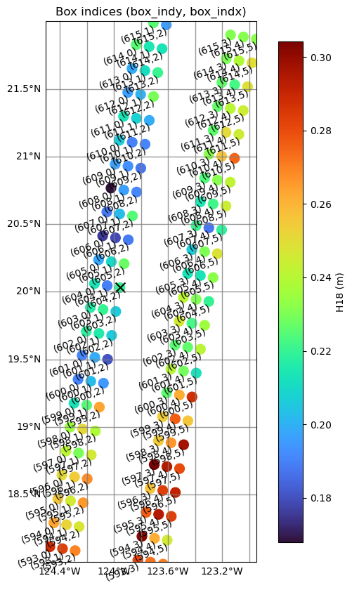
Using box indices to get original SSHA
The variables box_indx and box_indy are provided to locate the position of each box within the swath, corresponding to the cross-track and along-track directions, respectively.
The box_indx values are defined as follows:
0–1 for 40 km boxes (left or right swath)
0-5 for 20 km boxes (0–2 for the left swath and 3–5 for the right swath in the satellite frame)
0–13 for 10 km boxes (0–6 for the left swath and 7–13 for the right swath in the satellite frame)
See User handbook (section 2.2)
Show box indices
zoom_coords = [lon_start_plot, lon_stop_plot, lat_start_plot, lat_stop_plot]

central_lon = ds_sel['longitude'].values[ds_sel.sizes['n_box']//2]

f, ax = plt.subplots(
    1,
    1,
    figsize=(10,10),
    subplot_kw={'projection':ccrs.PlateCarree(central_longitude=central_lon)}
)

ax = custom_ax(ax, extent=zoom_coords)

im = ax.scatter(
    ds_sel.longitude,
    ds_sel.latitude,
    c= ds_sel['H18'],
    s=100,
    cmap='turbo',
    transform=ccrs.PlateCarree()
)
cbar = plt.colorbar(im, ax=ax,
    fraction=0.046, pad=0.04)
cbar.set_label('H18 (m)')

for box_y, box_x, lat, lon in zip(ds_sel['box_indy'].values, \
                                  ds_sel['box_indx'].values, \
                                  ds_sel['latitude'].values, \
                                  ds_sel['longitude'].values):
    if (zoom_coords[2]<=lat) & (zoom_coords[3]>=lat):
        ax.text(lon-0.25, lat-0.01,
                '(%d,%d)'%(box_y, box_x),
            verticalalignment='top',
            rotation = 20,
            transform=ccrs.PlateCarree())
    else:
        continue

ax.scatter(
    ds_sel.longitude[ind],
    ds_sel.latitude[ind],
    marker='x',
    s=100,
    c='k',
    transform=ccrs.PlateCarree()
)

ax.set_title('Box indices (box_indy, box_indx)')

plt.show()
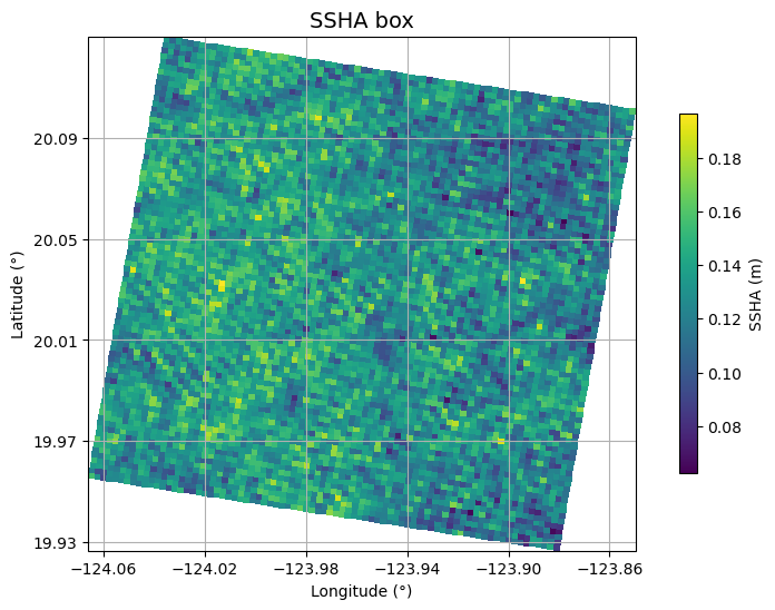
Get original SSHA
Plot SSH from L3 SSH product used for estimating spectra in L3 WW product
box_indices = ds_sel['box_indices'][ind].values.astype(int)
alti_data = AltimetryData(
    source=FileCollectionSource(
        path=output_dir,
        ftype="SWOT_L3_LR_SSH",
        subset="Unsmoothed"
    ),
)
ds_ssh = alti_data.query_orbit(
    cycle_number=cycle_number,
    pass_number=pass_number,
    variables=['latitude', 'longitude', 'ssha_unfiltered', 'quality_flag']
)
ds_ssh
INFO:fcollections.core._readers:Files to read: 1
<xarray.Dataset> Size: 1GB
Dimensions:          (num_lines: 82966, num_pixels: 519)
Coordinates:
    latitude         (num_lines, num_pixels) float64 344MB dask.array<chunksize=(4000, 260), meta=np.ndarray>
    longitude        (num_lines, num_pixels) float64 344MB dask.array<chunksize=(4000, 260), meta=np.ndarray>
Dimensions without coordinates: num_lines, num_pixels
Data variables:
    quality_flag     (num_lines, num_pixels) uint8 43MB dask.array<chunksize=(4000, 260), meta=np.ndarray>
    ssha_unfiltered  (num_lines, num_pixels) float64 344MB dask.array<chunksize=(4000, 260), meta=np.ndarray>
    cycle_number     (num_lines) uint16 166kB 6 6 6 6 6 6 6 6 ... 6 6 6 6 6 6 6
    pass_number      (num_lines) uint16 166kB 567 567 567 567 ... 567 567 567
Attributes: (12/42)
    Conventions:                     CF-1.7
    Metadata_Conventions:            Unidata Dataset Discovery v1.0
    cdm_data_type:                   Swath
    comment:                         Sea Surface Height measured by Altimetry
    data_used:                       SWOT KaRIn L2_LR_SSH PGC0/PIC0 (NASA/CNE...
    doi:                             https://doi.org/10.24400/527896/A01-2024...
    ...                              ...
    geospatial_lon_min:              149.669041
    geospatial_lon_max:              316.718346
    date_modified:                   2025-03-07T04:39:51Z
    history:                         2025-03-07T04:39:51Z: Created by DUACS K...
    date_created:                    2025-03-07T04:39:51Z
date_issued: 2025-03-07T04:39:51Zbox_ssh = ds_ssh.isel(num_lines=slice(box_indices[0],box_indices[1]), num_pixels=slice(box_indices[2],box_indices[3]))
box_ssh['longitude'] = (box_ssh['longitude'] + 180)%360 - 180
box_ssh['ssha_filtered'] = box_ssh['ssha_unfiltered'].where(
            (box_ssh['quality_flag'] == 0)
            |(box_ssh['quality_flag'] == 10)
            |(box_ssh['quality_flag'] == 20))

fig = plt.figure(figsize=(10, 6))
ax = plt.axes(projection=ccrs.PlateCarree())

ax.add_feature(cfeature.COASTLINE, linewidth=0.5)
ax.add_feature(cfeature.BORDERS, linestyle=":", linewidth=0.5)
ax.add_feature(cfeature.LAND, facecolor="lightgray")

im = ax.pcolormesh(
    box_ssh.longitude,
    box_ssh.latitude,
    box_ssh['ssha_filtered'],
    transform=ccrs.PlateCarree()
)

cbar = plt.colorbar(im, orientation="vertical", ax=ax, shrink=0.7, label="SSHA (m)")

ax.set_title("SSHA box", fontsize=14)
ax.set_xlabel("Longitude (°)")
ax.set_ylabel("Latitude (°)")
xticks = np.arange(np.round(np.min(box_ssh.longitude),2),
                   np.round(np.max(box_ssh.longitude),2),
                   0.04)
yticks = np.arange(np.round(np.min(box_ssh.latitude),2),
                   np.round(np.max(box_ssh.latitude),2),
                   0.04)
ax.set_xticks(xticks)
ax.set_yticks(yticks)
ax.grid()

plt.show()
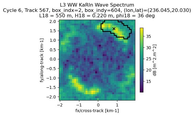
Plot KaRIn spectrum
SSHA-based 2-dimensional wave spectra, for waves with periods longer than ~500 m (18 s)
Unsmoothed KaRIn data has a spatial posting of ~250 m so the smallest observable wavelength is ~500 m, which is equivalent to ~18 s through the wave dispersion equation. For this reason, integrated wave parameters are denoted with the suffix “18” as 𝐻18 (significant wave height), 𝐿18 (wavelength) and ϕ_18 (wave direction).
The estimation of the wave heights PSD starts with the computation of the KaRIn SSHA power spectral density. The estimation is performed for each spatial box.
See User handbook (section 2.3)
Plot KaRIn spectrum provided in cartesian coordinates
Express frequencies in km-1
fx2 = ds_box['fx2D'].values*1e3
fy2 = ds_box['fy2D'].values*1e3
Get mask and integrated wave parameters
xmask, ymask = get_mask_border(
    ds_sel['swell_mask'][ind].values,
    fx2[0,:],
    fy2[:,0]
)
L18 = ds_sel['L18'][ind].values*1e-3 # in km
phi18_NE = ds_sel['phi18'][ind].values
H18 = ds_sel['H18'][ind].values
Get wave direction in SWOT reference system
phi18_SWOT = rotate_angle_from_NE_to_SWOT_ref_system(
    phi18_NE,
    ds_sel['track_angle'][ind].values
)
Plot
fig, ax = plt.subplots(nrows=1, ncols=1,figsize=(4.1, 3.5))
im=ax.pcolormesh(
    fx2,
    fy2,
    10*np.log10(ds_sel['Efxfy_SWOT'][ind].values),
    cmap='viridis',
    rasterized=True
)
ax.set_xlabel("fx/cross-track [km-1]")
ax.set_ylabel("fy/along-track [km-1]")
cbar=plt.colorbar(im,ax=ax,label='dB [m^2.m^2]', shrink=0.8)

# Plot mask and swell barycenter
ax.plot(xmask, ymask, linewidth=2, color='k')
ax.scatter(
    1/L18*np.sin(np.deg2rad(phi18_SWOT)),
    1/L18*np.cos(np.deg2rad(phi18_SWOT)),
    marker = 'x',
    color = 'k'
)
info_sample_str = 'Cycle %d, Track %d, box_indx=%d, box_indy=%d, (lon,lat)=(%.3f,%.3f)\n'% (cycle_number,
                                                                 pass_number,
                                                                 ds_sel['box_indx'][ind].values,
                                                                 ds_sel['box_indy'][ind].values,
                                                                 ds_sel['longitude'][ind].values,
                                                                 ds_sel['latitude'][ind].values) + \
                    'L18 = %d m, H18 = %.3f m, phi18 = %d deg' % (L18*1e3,
                                                                    H18,
                                                                    phi18_NE
                                                                    )
ax.set_title('L3 WW KaRIn Wave Spectrum\n' + info_sample_str)
plt.show()
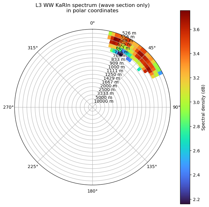
Plot KaRIn spectrum provided in polar coordinates
ds_box.load()
<xarray.Dataset> Size: 615MB
Dimensions:              (nfy: 42, nfx: 40, nphi: 144, nf: 20, n_box: 5922,
                          nind: 4)
Coordinates:
    longitude            (n_box) float64 47kB 150.1 150.1 ... -44.24 -44.24
    latitude             (n_box) float64 47kB -77.27 -77.36 ... 77.36 77.27
Dimensions without coordinates: nfy, nfx, nphi, nf, n_box, nind
Data variables: (12/33)
    filter_PTR           (nfy, nfx) float64 13kB 0.2415 0.2415 ... 0.2685 0.2685
    phi_vector           (nphi) float64 1kB 0.0 0.04363 0.08727 ... 6.196 6.24
    fx2D                 (nfy, nfx) float64 13kB -0.002 -0.0019 ... 0.0019
    f_vector             (nf) float64 160B 0.0 0.0001 0.0002 ... 0.0018 0.0019
    fy2D                 (nfy, nfx) float64 13kB -0.002128 ... 0.002026
    filter_OBP           (nfy, nfx) float64 13kB 0.0008937 0.00129 ... 0.001844
    ...                   ...
    longitude_model      (n_box) float64 47kB nan nan nan nan ... nan nan nan
    time                 (n_box) datetime64[ns] 47kB 2023-11-22T18:38:15.0894...
    time_model           (n_box) datetime64[ns] 47kB NaT NaT NaT ... NaT NaT NaT
    phi18_model          (n_box) float64 47kB nan nan nan nan ... nan nan nan
    Hs_model             (n_box) float64 47kB nan nan nan nan ... nan nan nan
Efxfy_SWOT (n_box, nfy, nfx) float64 80MB nan nan nan ... nan nanf = ds_box.f_vector.data
phi = ds_box.phi_vector.data
S_fphi = ds_sel.isel(n_box=ind).E_f_phi_SWOT_masked.data
# Étendre les axes pour pcolormesh
F = np.linspace(f.min(), f.max(), len(f) + 1)
PHI = np.linspace(phi.min(), phi.max(), len(phi) + 1)
F_grid, PHI_grid = np.meshgrid(F, PHI, indexing="ij")
fig, ax = plt.subplots(subplot_kw={'projection': 'polar'}, figsize=(8, 8))
plot = ax.pcolormesh(PHI_grid, F_grid, np.log10(S_fphi), shading='flat', cmap='turbo')
plt.colorbar(plot, label="Spectral density (dB)")
f_ticks = f[1:]
T_ticks = 1 / f_ticks
ax.set_yticks(f_ticks)
ax.set_yticklabels([f"{T:.0f} m" for T in T_ticks])
ax.set_theta_zero_location("N")
ax.set_theta_direction(-1)
ax.set_title("L3 WW KaRIn spectrum (wave section only)\nin polar coordinates", pad=20)
plt.show()
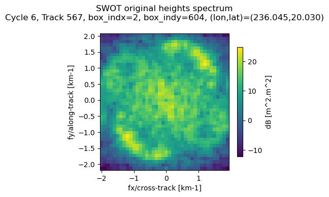
Undo KaRIn instrument corrections (show original KaRIn spectrum)
At the end of the processing chain, the KaRIn SSHA power spectral density (i.e. the “wave spectrum”) is corrected by dividing it by an approximation of the KaRIn transfer function. This one accounts mainly for the azimuth point target response (PTR), the on-board averaging filters and the azimuth cutoff effect. This correction is done on the assumption that the KaRIn processing is linear and many other considerations have been omitted (see handbook). For this reason, the user should have this in mind when using KaRIn corrected wave spectra.
The corrected spectrum if provided in both the Light and the Extended files. In addition, the Extended product provides the KaRIn transfer function correction, so the user can undo the correction if necessary (note that the filter aliasing cannot be undone, but this should not change the interpretation of results).
S_swot_original = ds_sel['Efxfy_SWOT'][ind].values * \
                  ds_box['filter_OBP'].values * \
                  ds_box['filter_PTR'].values * \
                  np.exp(-((fy2/1e3 * ds_sel['lambdac_model'][ind].values) ** 2)) # restore fy into m-1 (lambdac is given in m)
fig, ax = plt.subplots(nrows=1, ncols=1,figsize=(4.1, 3.5))
im=ax.pcolormesh(
    fx2,
    fy2,
    10*np.log10(S_swot_original),
    cmap='viridis',
    rasterized=True
)
ax.set_xlabel("fx/cross-track [km-1]")
ax.set_ylabel("fy/along-track [km-1]")
cbar=plt.colorbar(
    im,
    ax=ax,
    label='dB [m^2.m^2]',
    shrink=0.8
)

info_sample_str = 'Cycle %d, Track %d, box_indx=%d, box_indy=%d, (lon,lat)=(%.3f,%.3f)\n'% (cycle_number,
                                                                 pass_number,
                                                                 ds_sel['box_indx'][ind].values,
                                                                 ds_sel['box_indy'][ind].values,
                                                                 ds_sel['longitude'][ind].values,
                                                                 ds_sel['latitude'][ind].values)
ax.set_title('SWOT original heights spectrum\n' + info_sample_str)
plt.show()