Sea Ice Classification and local Leads/floes PDF analysis
This tutorial provides a step-by-step guide to analyzing polar region using SWOT data. It focuses on visualizing sea ice classification, binning ice concentration, and estimating ice freeboard (snow + ice thickness) using 2D histograms (Probability Density Functions, or PDFs).
Tutorial Objectives
Download Swot data with cycle/passes numbers, using
altimetry_downloader_avisoSelect data intersecting a geographical area, using
altimetry.ioPerform coordinates reprojection to ESPG:6931 using
pyprojVisualise sea ice classification using
matplotlib+cartopyPerform 2D binning on ice concentration, using
pyinterpEstimate ice freeboard using 2D histograms using
numpy+matplotlib
Note
Required environment to run this notebook:
xarray+numpypyprojgeopandas+shapelypyinterp+dask+numbamatplotlib+cartopyaltimetry_downloader_aviso: see documentation.altimetry.io: available here.
Import + code
import warnings
import numpy as np
import xarray as xr
import os
from pathlib import Path

import pyinterp

from pyproj import Proj, Transformer, transform

import matplotlib.pyplot as plt
import cartopy.crs as ccrs
from mpl_toolkits.axes_grid1 import make_axes_locatable
import matplotlib.axes as maxes
import logging
logging.basicConfig(level=logging.INFO)
def reproj_coords(ds, crs):
    """
    Transforms coordinates to a new crs
    """
    lat = ds["latitude"].values
    idx = np.where(lat >= LAT_BOUND)
    (_id, _) = idx
    sel = {'num_lines': slice(_id[0], _id[-1] + 1)}
    ds_crop = ds.isel(**sel)

    transformer = Transformer.from_crs(4326, crs)
    x_proj, y_proj = transformer.transform(
        ds_crop.latitude.data,
        ds_crop.longitude.data
    )
    ds_crop = ds_crop.assign(
        x_proj=(ds_crop.latitude.dims, x_proj),
        y_proj=(ds_crop.latitude.dims, y_proj)
    )
    return ds_crop
def set_carto(extent=None, nrows=1, ncols=1, projection=ccrs.NorthPolarStereo(), central_lon=0, figsize=(14, 12)):

    fig, axs = plt.subplots(
        nrows=nrows,
        ncols=ncols,
        subplot_kw={'projection':projection},
        figsize=figsize,
        dpi=80
    )
    gl = axs.gridlines(draw_labels=True)
    gl.top_labels = gl.right_labels = False
    axs.coastlines(color="black", lw=0.5)
    divider = make_axes_locatable(axs)
    ax_cb = divider.new_horizontal(size="5%", pad=0.1, axes_class=plt.Axes)
    fig = plt.gcf()
    fig.add_axes(ax_cb)
    if extent:
        axs.set_extent(extent, crs=ccrs.PlateCarree())

    return fig, axs, ax_cb

def get_bins(lat_bound: float, resolution: float):
    """
    Generates a regular grid (xc_bins, yc_bins) in North polar stereographical projection
    """
    proj_polar = Proj(proj='stere', lat_0=90, lat_ts=70, lon_0=-45, datum='WGS84', units='m')

    x_min, y_min = proj_polar(0, lat_bound)
    x_max, y_max = 0, 0
    dist_max = np.abs(y_min)

    extent = dist_max
    num_bins = int(np.ceil((2 * extent) / resolution)) + 1

    xc_bins = np.linspace(-extent, extent, num_bins)
    yc_bins = np.linspace(-extent, extent, num_bins)

    return xc_bins, yc_bins

def plot_ice_conc(Xgeo, Ygeo, bin2d, crs, extent, central_latitude, fig_title, figsize=(10,15)):

    fig = plt.figure(figsize=figsize)
    ax = plt.axes(projection=ccrs.LambertAzimuthalEqualArea(central_latitude=central_latitude))

    ax.coastlines()
    ax.set_extent(extent, crs=ccrs.PlateCarree())
    gl = ax.gridlines(crs=ccrs.PlateCarree(), draw_labels=True,
                      linewidth=2, color='gray', alpha=0.5, linestyle='--')

    im = ax.pcolormesh(
        Xgeo,
        Ygeo,
        (1-bin2d.variable("mean")).T*100,
        transform=ccrs.epsg(crs),
        vmin=0,
        vmax=100,
        cmap="Spectral_r"
    )

    divider = make_axes_locatable(ax)
    cax = divider.append_axes("bottom", "3%", pad='7%', axes_class=maxes.Axes)
    plt.colorbar(im, label='Sea ice concentration [%]', cax=cax, location='bottom')

    ax.set_title(f"{fig_title} \n Mean sure leads (3) to sure leads and floes (3 and 0)\n1 and 2 values are ignored")
Parameters
output_dir= Path.home() / "TMP_DATA"

cycle_number=[13]
half_orbits = [153, 155, 157, 181, 183, 209, 211, 237, 239, 265, 267, 291, 293, 295]

bbox=(-151, -109, 71, 78)

# coverage and resolution
LAT_BOUND = 60        # min absolute latitude
RESOLUTION = 12500.    # pixels size in meters
Download data using altimetry_downloader_aviso
import altimetry_downloader_aviso as dl_aviso
dl_aviso.get(
    'SWOT_L3_LR_SSH_Unsmoothed',
    output_dir=output_dir,
    cycle_number=cycle_number,
    pass_number=half_orbits,
)
INFO:altimetry_downloader_aviso.catalog_client.client:Fetching products from Aviso's catalog...
INFO:altimetry_downloader_aviso.catalog_client.granule_discoverer:Filtering SWOT_L3_LR_SSH_Unsmoothed product with filters {'cycle_number': [13], 'pass_number': [153, 155, 157, 181, 183, 209, 211, 237, 239, 265, 267, 291, 293, 295]}...
INFO:altimetry_downloader_aviso.core:14 files to download. 0 files already exist.
INFO:altimetry_downloader_aviso.tds_client:File /home/atonneau/TMP_DATA/SWOT_L3_LR_SSH_Unsmoothed_013_153_20240402T005441_20240402T014608_v2.0.1.nc downloaded.
INFO:altimetry_downloader_aviso.tds_client:File /home/atonneau/TMP_DATA/SWOT_L3_LR_SSH_Unsmoothed_013_155_20240402T023735_20240402T032902_v2.0.1.nc downloaded.
INFO:altimetry_downloader_aviso.tds_client:File /home/atonneau/TMP_DATA/SWOT_L3_LR_SSH_Unsmoothed_013_157_20240402T042028_20240402T051153_v2.0.1.nc downloaded.
INFO:altimetry_downloader_aviso.tds_client:File /home/atonneau/TMP_DATA/SWOT_L3_LR_SSH_Unsmoothed_013_181_20240403T005512_20240403T014639_v2.0.1.nc downloaded.
INFO:altimetry_downloader_aviso.tds_client:File /home/atonneau/TMP_DATA/SWOT_L3_LR_SSH_Unsmoothed_013_183_20240403T023806_20240403T032932_v2.0.1.nc downloaded.
INFO:altimetry_downloader_aviso.tds_client:File /home/atonneau/TMP_DATA/SWOT_L3_LR_SSH_Unsmoothed_013_209_20240404T005543_20240404T014710_v2.0.1.nc downloaded.
INFO:altimetry_downloader_aviso.tds_client:File /home/atonneau/TMP_DATA/SWOT_L3_LR_SSH_Unsmoothed_013_211_20240404T023836_20240404T033001_v2.0.1.nc downloaded.
INFO:altimetry_downloader_aviso.tds_client:File /home/atonneau/TMP_DATA/SWOT_L3_LR_SSH_Unsmoothed_013_237_20240405T005614_20240405T014741_v2.0.1.nc downloaded.
INFO:altimetry_downloader_aviso.tds_client:File /home/atonneau/TMP_DATA/SWOT_L3_LR_SSH_Unsmoothed_013_239_20240405T023907_20240405T033032_v2.0.1.nc downloaded.
INFO:altimetry_downloader_aviso.tds_client:File /home/atonneau/TMP_DATA/SWOT_L3_LR_SSH_Unsmoothed_013_265_20240406T005645_20240406T014812_v2.0.1.nc downloaded.
INFO:altimetry_downloader_aviso.tds_client:File /home/atonneau/TMP_DATA/SWOT_L3_LR_SSH_Unsmoothed_013_267_20240406T023938_20240406T033105_v2.0.1.nc downloaded.
INFO:altimetry_downloader_aviso.tds_client:File /home/atonneau/TMP_DATA/SWOT_L3_LR_SSH_Unsmoothed_013_291_20240406T231422_20240407T000508_v2.0.1.nc downloaded.
INFO:altimetry_downloader_aviso.tds_client:File /home/atonneau/TMP_DATA/SWOT_L3_LR_SSH_Unsmoothed_013_293_20240407T005716_20240407T014843_v2.0.1.nc downloaded.
INFO:altimetry_downloader_aviso.tds_client:File /home/atonneau/TMP_DATA/SWOT_L3_LR_SSH_Unsmoothed_013_295_20240407T024010_20240407T033136_v2.0.1.nc downloaded.
['/home/atonneau/TMP_DATA/SWOT_L3_LR_SSH_Unsmoothed_013_153_20240402T005441_20240402T014608_v2.0.1.nc',
 '/home/atonneau/TMP_DATA/SWOT_L3_LR_SSH_Unsmoothed_013_155_20240402T023735_20240402T032902_v2.0.1.nc',
 '/home/atonneau/TMP_DATA/SWOT_L3_LR_SSH_Unsmoothed_013_157_20240402T042028_20240402T051153_v2.0.1.nc',
 '/home/atonneau/TMP_DATA/SWOT_L3_LR_SSH_Unsmoothed_013_181_20240403T005512_20240403T014639_v2.0.1.nc',
 '/home/atonneau/TMP_DATA/SWOT_L3_LR_SSH_Unsmoothed_013_183_20240403T023806_20240403T032932_v2.0.1.nc',
 '/home/atonneau/TMP_DATA/SWOT_L3_LR_SSH_Unsmoothed_013_209_20240404T005543_20240404T014710_v2.0.1.nc',
 '/home/atonneau/TMP_DATA/SWOT_L3_LR_SSH_Unsmoothed_013_211_20240404T023836_20240404T033001_v2.0.1.nc',
 '/home/atonneau/TMP_DATA/SWOT_L3_LR_SSH_Unsmoothed_013_237_20240405T005614_20240405T014741_v2.0.1.nc',
 '/home/atonneau/TMP_DATA/SWOT_L3_LR_SSH_Unsmoothed_013_239_20240405T023907_20240405T033032_v2.0.1.nc',
 '/home/atonneau/TMP_DATA/SWOT_L3_LR_SSH_Unsmoothed_013_265_20240406T005645_20240406T014812_v2.0.1.nc',
 '/home/atonneau/TMP_DATA/SWOT_L3_LR_SSH_Unsmoothed_013_267_20240406T023938_20240406T033105_v2.0.1.nc',
 '/home/atonneau/TMP_DATA/SWOT_L3_LR_SSH_Unsmoothed_013_291_20240406T231422_20240407T000508_v2.0.1.nc',
 '/home/atonneau/TMP_DATA/SWOT_L3_LR_SSH_Unsmoothed_013_293_20240407T005716_20240407T014843_v2.0.1.nc',
 '/home/atonneau/TMP_DATA/SWOT_L3_LR_SSH_Unsmoothed_013_295_20240407T024010_20240407T033136_v2.0.1.nc']
Open data using altimetry.io
from altimetry.io import AltimetryData, FileCollectionSource
Open data source
alti_data = AltimetryData(
    source=FileCollectionSource(
        path=output_dir,
        ftype="SWOT_L3_LR_SSH",
        subset="Unsmoothed"
    ),
)
Query data
ds = alti_data.query_orbit(
    cycle_number=cycle_number,
    pass_number=half_orbits,
    variables=["time", "latitude", "longitude", "quality_flag", "ssha_unedited"],
    polygon=bbox
)
ds
INFO:fcollections.implementations.optional._predicates:The bbox intersects with pass numbers (calval phase): [1, 2, 3, 4, 5, 6, 7, 8, 9, 10, 11, 12, 13, 14, 15, 16, 17, 18, 19, 20, 21, 22, 23, 24, 25, 26, 27, 28]
INFO:fcollections.implementations.optional._predicates:The bbox intersects with pass numbers (science phase): [1, 2, 3, 4, 5, 6, 7, 8, 9, 10, 11, 12, 13, 14, 15, 16, 17, 18, 19, 20, 21, 22, 23, 24, 25, 26, 27, 28, 29, 30, 31, 32, 33, 34, 35, 36, 37, 38, 39, 40, 41, 42, 43, 44, 45, 46, 47, 48, 49, 50, 51, 52, 53, 54, 55, 56, 57, 58, 59, 60, 61, 62, 63, 64, 65, 66, 67, 68, 69, 70, 71, 72, 73, 74, 75, 76, 77, 78, 79, 80, 81, 82, 83, 84, 85, 86, 87, 88, 89, 90, 91, 92, 93, 94, 95, 96, 97, 98, 99, 100, 101, 102, 103, 104, 105, 106, 107, 108, 109, 110, 111, 112, 113, 114, 115, 116, 117, 118, 119, 120, 121, 122, 123, 124, 125, 126, 127, 128, 129, 130, 131, 132, 133, 134, 135, 136, 137, 138, 139, 140, 141, 142, 143, 144, 145, 146, 147, 148, 149, 150, 151, 152, 153, 154, 155, 156, 157, 158, 159, 160, 161, 162, 163, 164, 165, 166, 167, 168, 169, 170, 171, 172, 173, 174, 175, 176, 177, 178, 179, 180, 181, 182, 183, 184, 185, 186, 187, 188, 189, 190, 191, 192, 193, 194, 195, 196, 197, 198, 199, 200, 201, 202, 203, 204, 205, 206, 207, 208, 209, 210, 211, 212, 213, 214, 215, 216, 217, 218, 219, 220, 221, 222, 223, 224, 225, 226, 227, 228, 229, 230, 231, 232, 233, 234, 235, 236, 237, 238, 239, 240, 241, 242, 243, 244, 245, 246, 247, 248, 249, 250, 251, 252, 253, 254, 255, 256, 257, 258, 259, 260, 261, 262, 263, 264, 265, 266, 267, 268, 269, 270, 271, 272, 273, 274, 275, 276, 277, 278, 279, 280, 281, 282, 283, 284, 285, 286, 287, 288, 289, 290, 291, 292, 293, 294, 295, 296, 297, 298, 299, 300, 301, 302, 303, 304, 305, 306, 307, 308, 309, 310, 311, 312, 313, 314, 315, 316, 317, 318, 319, 320, 321, 322, 323, 324, 325, 326, 327, 328, 329, 330, 331, 332, 333, 334, 335, 336, 337, 338, 339, 340, 341, 342, 343, 344, 345, 346, 347, 348, 349, 350, 351, 352, 353, 354, 355, 356, 357, 358, 359, 360, 361, 362, 363, 364, 365, 366, 367, 368, 369, 370, 371, 372, 373, 374, 375, 376, 377, 378, 379, 380, 381, 382, 383, 384, 385, 386, 387, 388, 389, 390, 391, 392, 393, 394, 395, 396, 397, 398, 399, 400, 401, 402, 403, 404, 405, 406, 407, 408, 409, 410, 411, 412, 413, 414, 415, 416, 417, 418, 419, 420, 421, 422, 423, 424, 425, 426, 427, 428, 429, 430, 431, 432, 433, 434, 435, 436, 437, 438, 439, 440, 441, 442, 443, 444, 445, 446, 447, 448, 449, 450, 451, 452, 453, 454, 455, 456, 457, 458, 459, 460, 461, 462, 463, 464, 465, 466, 467, 468, 469, 470, 471, 472, 473, 474, 475, 476, 477, 478, 479, 480, 481, 482, 483, 484, 485, 486, 487, 488, 489, 490, 491, 492, 493, 494, 495, 496, 497, 498, 499, 500, 501, 502, 503, 504, 505, 506, 507, 508, 509, 510, 511, 512, 513, 514, 515, 516, 517, 518, 519, 520, 521, 522, 523, 524, 525, 526, 527, 528, 529, 530, 531, 532, 533, 534, 535, 536, 537, 538, 539, 540, 541, 542, 543, 544, 545, 546, 547, 548, 549, 550, 551, 552, 553, 554, 555, 556, 557, 558, 559, 560, 561, 562, 563, 564, 565, 566, 567, 568, 569, 570, 571, 572, 573, 574, 575, 576, 577, 578, 579, 580, 581, 582, 583, 584]
INFO:fcollections.core._readers:Files to read: 14
INFO:fcollections.implementations.optional._area_selectors:Size of the dataset matching the bbox: {'num_lines': 14200, 'num_pixels': 519}
INFO:fcollections.implementations.optional._area_selectors:Size of the dataset matching the bbox: {'num_lines': 1693, 'num_pixels': 519}
INFO:fcollections.implementations.optional._area_selectors:Size of the dataset matching the bbox: {'num_lines': 3051, 'num_pixels': 519}
INFO:fcollections.implementations.optional._area_selectors:Size of the dataset matching the bbox: {'num_lines': 12665, 'num_pixels': 519}
INFO:fcollections.implementations.optional._area_selectors:Size of the dataset matching the bbox: {'num_lines': 913, 'num_pixels': 519}
INFO:fcollections.implementations.optional._area_selectors:Size of the dataset matching the bbox: {'num_lines': 11376, 'num_pixels': 519}
INFO:fcollections.implementations.optional._area_selectors:Size of the dataset matching the bbox: {'num_lines': 798, 'num_pixels': 519}
INFO:fcollections.implementations.optional._area_selectors:Size of the dataset matching the bbox: {'num_lines': 10279, 'num_pixels': 519}
INFO:fcollections.implementations.optional._area_selectors:Size of the dataset matching the bbox: {'num_lines': 2545, 'num_pixels': 519}
INFO:fcollections.implementations.optional._area_selectors:Size of the dataset matching the bbox: {'num_lines': 9330, 'num_pixels': 519}
INFO:fcollections.implementations.optional._area_selectors:Size of the dataset matching the bbox: {'num_lines': 1973, 'num_pixels': 519}
INFO:fcollections.implementations.optional._area_selectors:Size of the dataset matching the bbox: {'num_lines': 33187, 'num_pixels': 519}
INFO:fcollections.implementations.optional._area_selectors:Size of the dataset matching the bbox: {'num_lines': 8506, 'num_pixels': 519}
INFO:fcollections.implementations.optional._area_selectors:Size of the dataset matching the bbox: {'num_lines': 1400, 'num_pixels': 519}
<xarray.Dataset> Size: 1GB
Dimensions:        (num_lines: 111916, num_pixels: 519)
Coordinates:
    time           (num_lines) datetime64[ns] 895kB dask.array<chunksize=(14200,), meta=np.ndarray>
    latitude       (num_lines, num_pixels) float64 465MB dask.array<chunksize=(3950, 260), meta=np.ndarray>
    longitude      (num_lines, num_pixels) float64 465MB dask.array<chunksize=(3950, 260), meta=np.ndarray>
Dimensions without coordinates: num_lines, num_pixels
Data variables:
    quality_flag   (num_lines, num_pixels) uint8 58MB dask.array<chunksize=(3950, 260), meta=np.ndarray>
    ssha_unedited  (num_lines, num_pixels) float64 465MB dask.array<chunksize=(3950, 260), meta=np.ndarray>
    cycle_number   (num_lines) uint16 224kB 13 13 13 13 13 13 ... 13 13 13 13 13
    pass_number    (num_lines) uint16 224kB 153 153 153 153 ... 295 295 295 295
Attributes: (12/42)
    Conventions:                     CF-1.7
    Metadata_Conventions:            Unidata Dataset Discovery v1.0
    cdm_data_type:                   Swath
    comment:                         Sea Surface Height measured by Altimetry
    data_used:                       SWOT KaRIn L2_LR_SSH PGC0/PIC0 (NASA/CNE...
    doi:                             https://doi.org/10.24400/527896/A01-2024...
    ...                              ...
    geospatial_lon_min:              108.990992
    geospatial_lon_max:              275.949791
    date_modified:                   2025-03-06T20:03:00Z
    history:                         2025-03-06T20:03:00Z: Created by DUACS K...
    date_created:                    2025-03-06T20:03:00Z
date_issued: 2025-03-06T20:03:00Z1. Coordinates reprojection to ESPG:6931
# Arctic
crs = 6931
ds_proj = reproj_coords(ds, crs)
ds_proj
<xarray.Dataset> Size: 2GB
Dimensions:        (num_lines: 110575, num_pixels: 519)
Coordinates:
    time           (num_lines) datetime64[ns] 885kB dask.array<chunksize=(12859,), meta=np.ndarray>
    latitude       (num_lines, num_pixels) float64 459MB dask.array<chunksize=(2609, 260), meta=np.ndarray>
    longitude      (num_lines, num_pixels) float64 459MB dask.array<chunksize=(2609, 260), meta=np.ndarray>
Dimensions without coordinates: num_lines, num_pixels
Data variables:
    quality_flag   (num_lines, num_pixels) uint8 57MB dask.array<chunksize=(2609, 260), meta=np.ndarray>
    ssha_unedited  (num_lines, num_pixels) float64 459MB dask.array<chunksize=(2609, 260), meta=np.ndarray>
    cycle_number   (num_lines) uint16 221kB 13 13 13 13 13 13 ... 13 13 13 13 13
    pass_number    (num_lines) uint16 221kB 153 153 153 153 ... 295 295 295 295
    x_proj         (num_lines, num_pixels) float64 459MB -1.604e+06 ... -1.21...
    y_proj         (num_lines, num_pixels) float64 459MB 2.895e+06 ... 7.661e+05
Attributes: (12/42)
    Conventions:                     CF-1.7
    Metadata_Conventions:            Unidata Dataset Discovery v1.0
    cdm_data_type:                   Swath
    comment:                         Sea Surface Height measured by Altimetry
    data_used:                       SWOT KaRIn L2_LR_SSH PGC0/PIC0 (NASA/CNE...
    doi:                             https://doi.org/10.24400/527896/A01-2024...
    ...                              ...
    geospatial_lon_min:              108.990992
    geospatial_lon_max:              275.949791
    date_modified:                   2025-03-06T20:03:00Z
    history:                         2025-03-06T20:03:00Z: Created by DUACS K...
    date_created:                    2025-03-06T20:03:00Z
date_issued: 2025-03-06T20:03:00Z2. Visualization of Sea Ice Classification with Flag Application
Learn how to apply quality flags to filter and visualize sea ice classification data.
Understand how to identify and exclude artifacts for accurate analysis.
extent = [-109, -151, 71, 73]
fig, ax, cb = set_carto(extent)
cb.remove()
# 19 = "ice_unsure"
# 20 = "ice"
# 101 = "not_on_sea"
# 102 = "no_data"

flag_sea_ice = xr.where(
    (ds_proj.quality_flag==19) | (ds_proj.quality_flag==20),
    0,
    xr.where((ds_proj.quality_flag==101) | (ds_proj.quality_flag==102),
        np.nan, # not_on_sea, no_data -> nan
        1
    )
)

ax.pcolormesh(
    ds_proj.longitude,
    ds_proj.latitude,
    flag_sea_ice,
    transform=ccrs.PlateCarree(),
    cmap="Blues",
    vmin=0,
    vmax=2,
)

fig = plt.gcf()

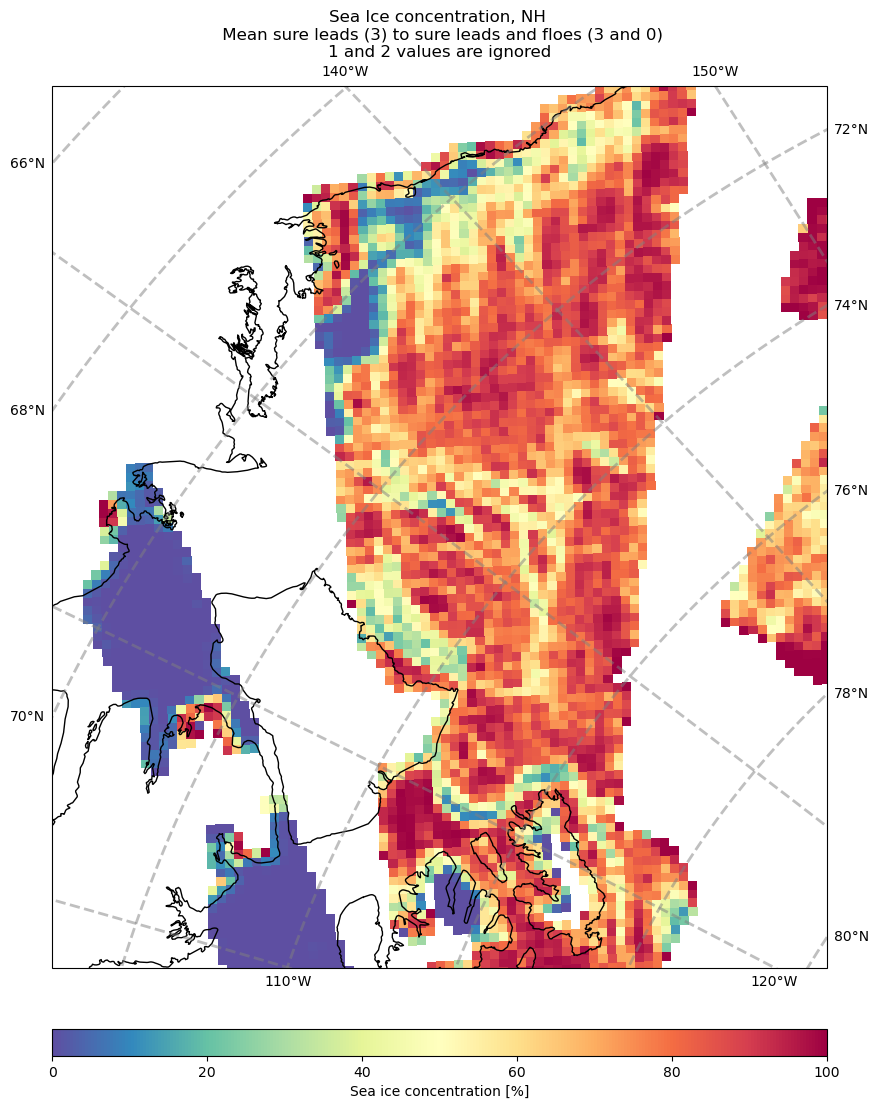
3. Binning and Visualization of Sea Ice Concentration
Perform spatial binning to visualize sea ice concentration.
Generate maps to highlight areas of interest for further analysis.
flag_sea_ice = xr.where(
    (ds_proj.quality_flag==20),
    0, # ice -> 0
    xr.where((ds_proj.quality_flag==101) | (ds_proj.quality_flag==102),
        np.nan, # not_on_sea, no_data -> nan
        1 # ice_unsure -> 1
    )
)
xc_bins, yc_bins = get_bins(LAT_BOUND, RESOLUTION)
x = ds_proj.x_proj.data.ravel()
y = ds_proj.y_proj.data.ravel()
z = flag_sea_ice.data.ravel()
x_axis = pyinterp.Axis(np.array(xc_bins, dtype='float64'))
y_axis = pyinterp.Axis(np.array(yc_bins, dtype='float64'))
bin2d_flag_ice_conc = pyinterp.Binning2D(x_axis, y_axis, dtype=np.dtype('float64'))
bin2d_flag_ice_conc.push(x, y, z, simple=False)
Plot result
central_latitude = 74
Xgeo, Ygeo = np.meshgrid(xc_bins, yc_bins)
fig_title = f'Sea Ice concentration, NH'

plot_ice_conc(Xgeo, Ygeo, bin2d_flag_ice_conc, crs, extent, central_latitude, fig_title)
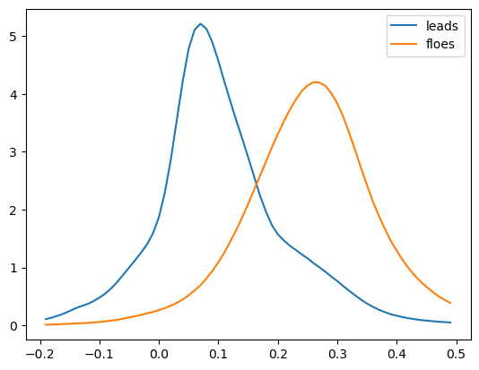
4. 2D Histogram (PDF) Analysis for Leads and Floes
Calculate 2D histograms (PDFs) for sea ice leads (cracks) and floes (ice sheets).
Compare the PDFs of leads and floes to derive differences in elevation.
Use the difference between the two PDFs to estimate the freeboard (snow + ice thickness) from SWOT KaRIn, with an expected order of magnitude of ~20 cm.
ssha_leads = xr.where(flag_sea_ice==1, ds_proj.ssha_unedited, np.nan)
ssha_floes = xr.where(flag_sea_ice==0, ds_proj.ssha_unedited, np.nan)
hist, bins = np.histogram(ssha_leads, bins=np.arange(-0.2,0.5,0.01), density=True)
hist_floes, bins = np.histogram(ssha_floes, bins=np.arange(-0.2,0.5,0.01), density=True)
plt.figure()
plt.plot(bins[1:],hist, label="leads")
plt.plot(bins[1:],hist_floes, label="floes")
plt.legend()
<matplotlib.legend.Legend at 0x76b6ec586d90>