Known limitations and anomalies

We list in this section the known limitations or anomalies observed in the L3 KaRIn products

Missing estuaries in land-sea mask

Some areas (especially estuaries) are not well defined in OpenStreetMap and will show land where we would expect sea.

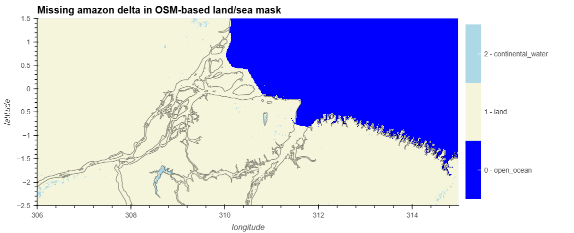
This issue has been mitigated:

• In V2.0 by blending the L2 mask over the identified problematic areas, which include 43 estuaries. Additionnal problematic areas spotted by the users might be communicated to aviso-swot@altimetry.fr for further patching.

• In V3.0 by introducing a new land-sea mask selection criterion

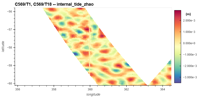
Internal Tide Discontinuity around 0°E

• Affected version: 3.0.0

• Affected subsets: Technical

The internal tide projection of Zhao, 2025 shows a discontinuity around longitude 0. This should be fixed in subsequent versions

Discrepancy of valid domains for FES22 corrections in v2.0 and v2.0.1

In some particular areas, users might observe that some of Level-3 data is missing with respect to Level-2 data, and that the quality flag investigation is marked as no_data

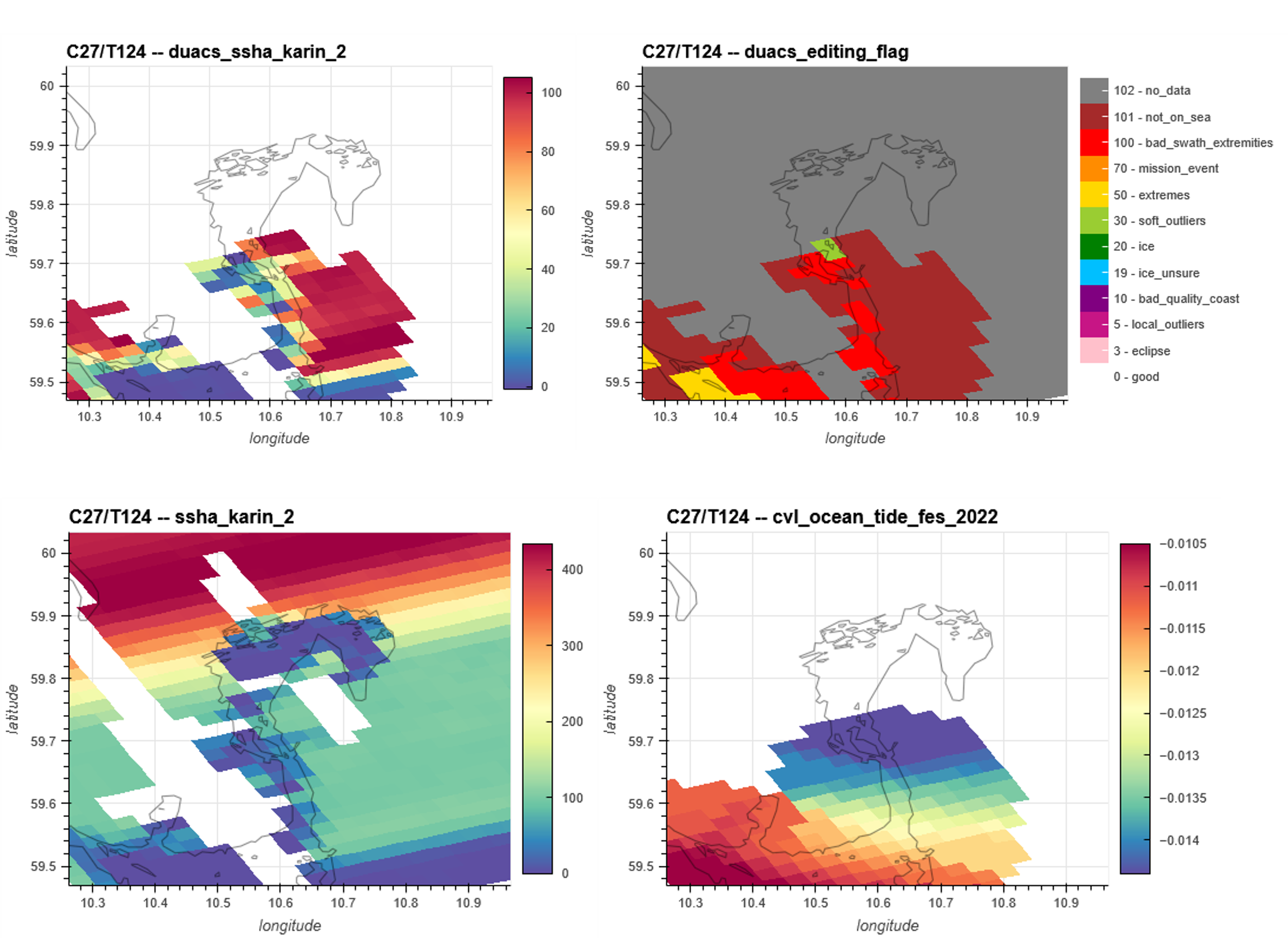
Missing points in L3 are observed when comparing the Sea Level Anomaly from Level-3 (top left) and Level-2 (bottom left) products. The quality flag (top right) indicates missing data in gray that are explained by missing data in the ocean tide correction (bottom right)

The missing data is introduced by the ocean tide correction FES 2022, which is not defined at the problematic location. Even if the ocean tide correction is the same in both the baseline C Level 2 product and the v2.0.1 Level 3 product, the source of the correction differs. Level-2 product uses an extrapolated cartesian grid whereas the Level-3 product uses the finite element meshes which has a smaller domain of definition. This is illustrated in the following figure:

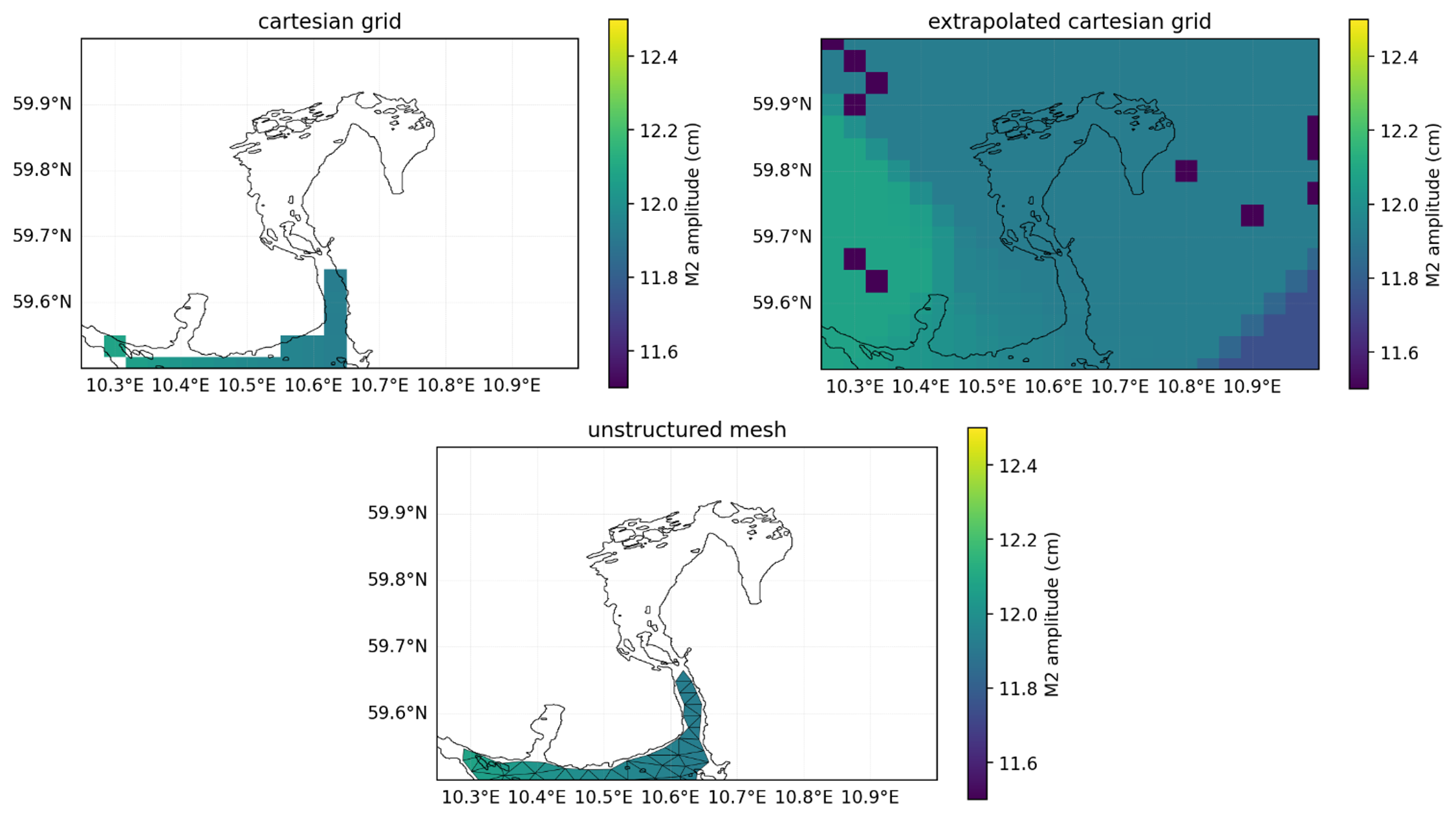
Difference in the definition of the FES2022 source data with (bottom) the original unstructured mesh used in the Level-3 product (top left) the cartesian grid interpolated from the mesh and (top right) the extrapolated cartesian grid used in the Level-2 product

This issue was mitigated in V3.0 by using the FES22 solution from extrapolated cartesian grid when the unstructured mesh solution is not available.

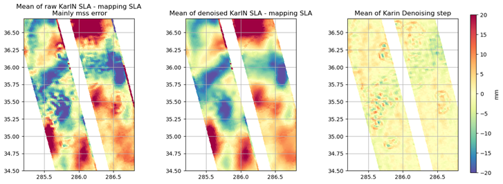
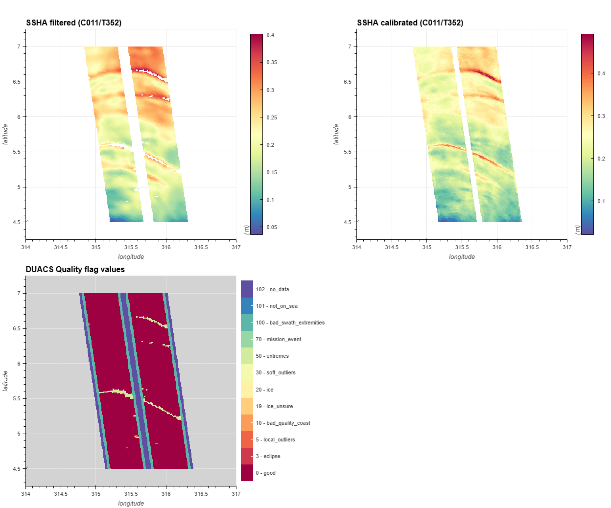
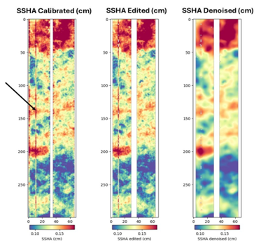
Use of ssha_filtered and MSS in V2.0 and V2.0.1

The analysis of the constant content of the noise removed with the filtering can underline statics small scales structures linked to the MSS field used for the SSHA computation (see example in the following figure). Consequently, we recommend to users that may want to use a different MSS field than the one used in the L3 processing to work with the “ssha_unfiltered” field (i.e. before denoising processing) rather than “ssha_filtered” (i.e. after denoising processing)

ssha_filtered biases and discontinuities in v2.0 and V2.0.1

Regional biases in the ssha_filtered product were observed, primarily in areas of high SWH, where they can reach several centimeters. These biases are identified as anomalies introduced during the denoising process and are likely due to limitations in the current noise-modeling scheme. These biases are also visible in regions of strong variability, such as the Gulf Stream. The denoising versions V2.0 and V2.0.1 can absorb part of the oceanic structures and sometimes even amplify them. These biases can be so strong that they create a discontinuity in the predicted swaths (see following figure, purple circle).

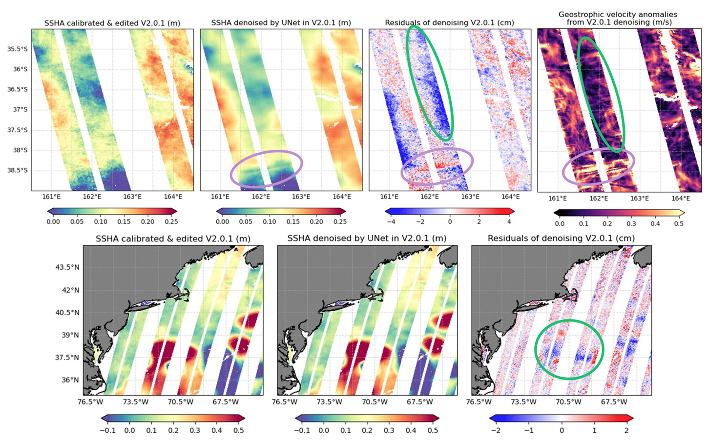
Example of regional biases induced by denoising processing in v2

Certain physical structures may be attenuated by the denoising process implemented in version V2, particularly those associated with short-wavelength wave signals. This phenomenon is illustrated in the following figure, where notable smoothing and signal loss are observed.

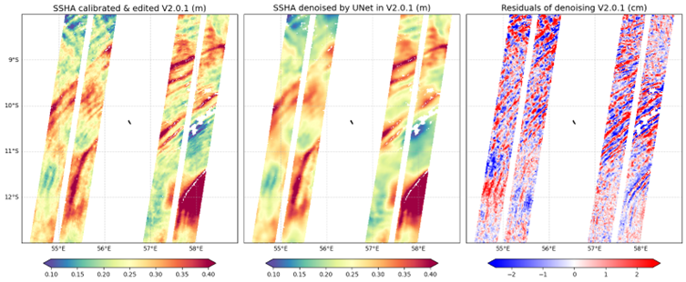
Example of waves attenuated by denoising processing in v2

These issues were mitigated in V3.0 by using an improved denoising

SSHA restrictive quality flag during extreme events in v2.0 and V2.0.1 : Example of Hurricane Milton

The cycle 22, pass 216 intersects with the path of Hurricane Milton. Some pixels are rejected with flag #30 (SSHa pixels out of the expected statistical distribution) and #5 (SSHa pixels out of local distribution). This is mainly due to rain cells. For scientists who want to work on the Hurricane or on similar cases, we suggest applying flags higher than 30 (quality_flag variable) on the ssha_unedited variable.

Example of Hurricane Milton. Left: ssha variable i.e. ssha with all flags applied. Middle: ssha with only flags > 30 applied. Right: quality flag

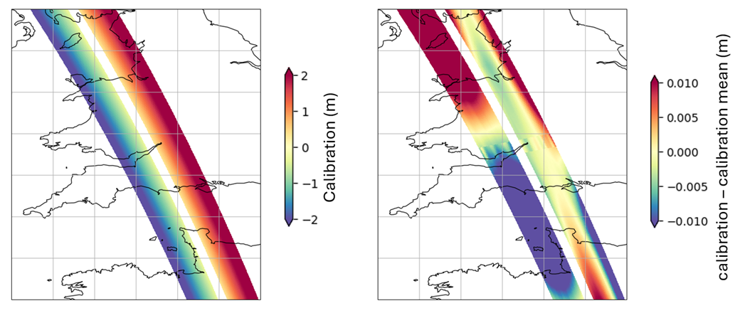
Small-scale discontinuities and errors in the calibration variable

• Affected versions: All

• Affected subsets: All

In some areas, when a L2 field (sc_yaw) is not defined, some small-scale terms of the calibration are reverted. This inversion causes small-scale discontinuities and errors inside the calibration variable. As these discontinuities and errors are small-scale, they are only visible if the calibration mean is removed. This issue only occurs when SSHA is not defined, thus this issue does not affect SSHA.

Wrong editing flag in Unsmoothed product during eclipse transition

Some eclipse transitions in the Unsmoothed product are flagged with flag 30 instead of flag 3. These eclipses are not kept in the edited and filtered SSHA. There is therefore inhomogeneity between the Expert and Unsmoothed products.

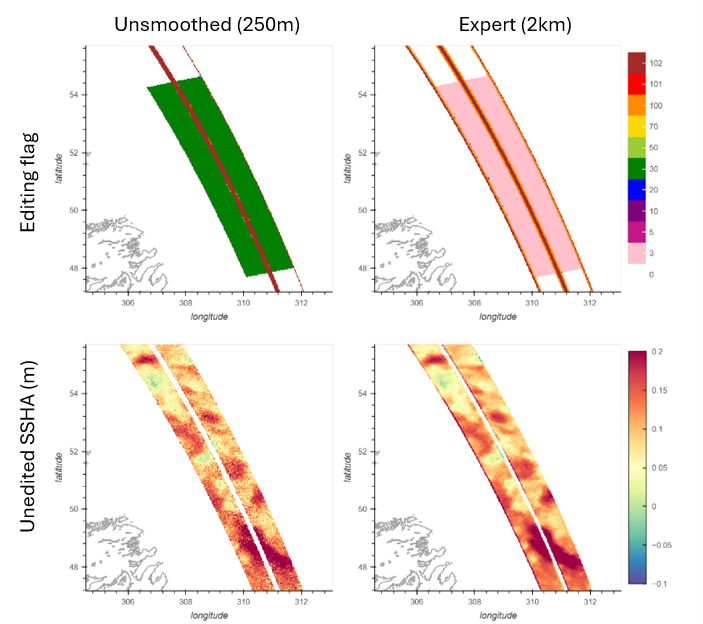
Example of eclipse transition with inhomogeneous flags between Expert and Unsmoothed products

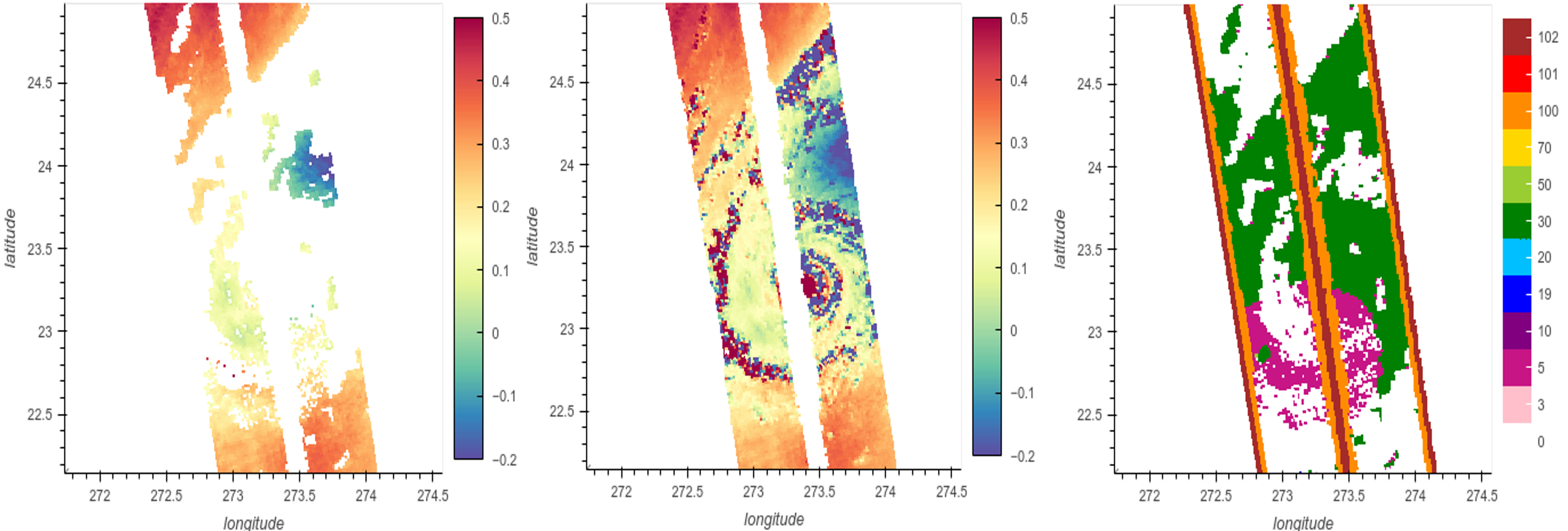
Wrong wave crest editing

Some soliton waves have a wrong editing. A visual check shows that the non-edited data seems normal, but the wave’s crest is still flagged as outside the expected Sea Surface Height distribution. Users can switch to the duacs_ssha_karin_2_calibrated variable and tune the diting following this tutorial

SSHA calibration discontinuity

• Affected versions: 3.0.0

• Affected subsets: All

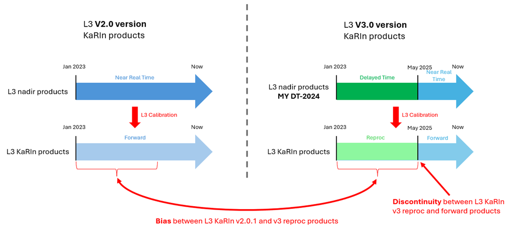
The calibration correction presents a discontinuity related with the residual biases observed between Copernicus Marine Service L3 nadir products available in delayed time (MY DT-2024 series) and in Near Real Time (NRT). Indeed, for version 1.0.2 and 2.0.1, the KaRIn L3 data were calibrated from the Copernicus Marine Service L3 nadir products available in NRT. For version 3.0, an upgrade has been made in order to use L3 nadir MY products when available. The Copernicus Marine Service L3 nadir products based on MY DT-2024 standard are available in delayed time until May 2024 and, then in NRT after that date. Time evolving global and regional biases exist between L3 nadir MY and NRT series.

The following figure (left) illustrates the biases observed between L3 nadir MY and NRT series used for the L3 KaRIn v3 calibration. These biases propagate into the KaRIn calibration results as illustrated in the figure (right).

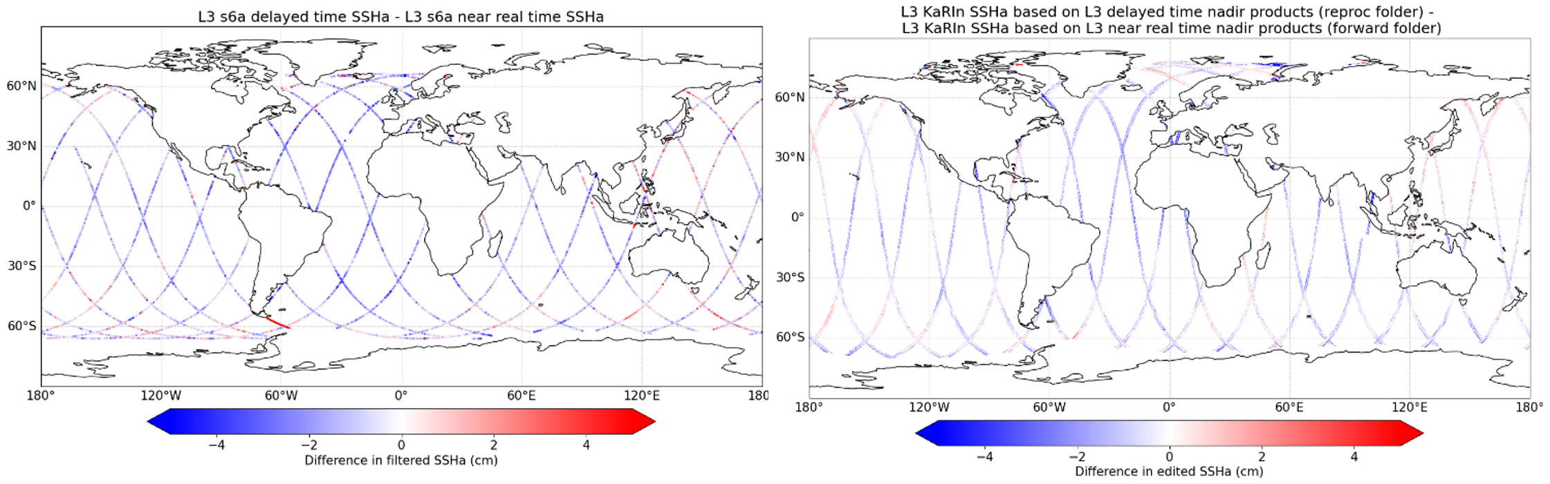
Bias between L3 s6a delayed time and near real time SSHa and its impacts on L3 KaRIn reproc and forward SSHA for the day of 2024/05/20

To differentiate between the two calibration periods (based on L3 nadir MY or NRT), the L3 v3 KaRIn products are distributed in two separate directories:

• The reproc directory which contains L3 KaRIn products calibrated from the Copernicus Marine Service L3 nadir products available in delayed time (MY DT-2024 series)

• The forward directory which contains L3 KaRIn products calibrated from the Copernicus Marine Service L3 nadir products available in NRT (DT-2024 standards)

Impact diagram of L3 nadir inputs on L3 KaRIn products

HRET22 limitation in v2 and v3

Some problems with the blending of HRET14 and HRET8.1 have been detected. They are especially apparent when considering the non-M2 constituents and are generally at the mm-amplitude level, but involve non-physical-looking wave patterns that arise from the blending. Actions are on going to solve the problems in a future version of HRET model.

In the meanwhile, users who observe some of these issues can use the Technical product to apply an alternative internal wave correction provided in this product (MIOST-IT24 and Zhao30y).

Along-track lines in V2 and in V3

As underlined by (Chen et Chen 2025), KaRIn on-board processor (OBP) is implemented using electronic field-programmable gate array (FPGA) chips that are somewhat susceptible to upset by ionizing radiation in space. An ionizing particle may cause one or more binary bits to be erroneously flipped. This is called a single event upset (SEU). This occurs at random times due to the radiation environment in low-Earth orbit. These phenomena start abruptly (but may start over land) and end when the on-board processor automatically resets itself to clear radiation corruption (“FPGA reconfig”). These anomalies remain visible in the L3 products, with a signature modified by the different processing steps. An example is shown in the following figure for LR 2km data

Impact of SEU event on L3 SSHA

We counted on phase SCIENCE the cycles and passes impacted. The list might not be complete:

• Cycle 3, Tracks 365 to 367

• Cycle 5, Tracks 478-479

• Cycle 6, Track 66

• Cycle 10, Tracks 33 to 39

• Cycle 12, Tracks 217 to 220

• Cycle 22, Tracks 218 to 221

• Cycle 32, Track 115

• Cycle 34, Track 171

• Cycle 35, Track 171

Unrealistic gradient dynamics on swaths border in case of large scale oceanic features

In V3.0 and previous versions, the computation of SSHA gradients (i.e. geostrophic velocities and relative vorticity) can lead to small errors on outside borders of the swath. This occurs especially when large-scale oceanic features are cut by the SWOT track. This issue is NOT related to denoising which performs as usual. It is related to the gradient computation method itself (e.g. stencil or 2D spline fitting, see section 2.7) that is struggling near borders. A different derivation method will lead to different results (see the following figure). Feel free to contact AVISO service desk if you use your own approach that you find more appropriate than the implemented ones, we would be delighted to implement it in the next products. We recommend the user to be careful when interpreting near swaths border relative vorticity with a linear and horizontal pattern as illustrated.

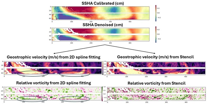
Errors of relative vorticity on swath border after 2D spline fitting derivation method that we do not see using Stencil (but it can occurs with stencil too)

Bias anomaly caused by L3 calibration in passes parallel to the coast

The L3 calibration parameters are calculated only for fully defined across-track lines. Passes parallel to the coastline include across-track lines that are not fully defined, for which the calibration parameters are not calculated but interpolated. This interpolation can cause locally degraded results, particularly for the bias parameter. In the next figure, we can see that at the crossover, there is a strong bias between the two passes, resulting from a bias problem on the pass parallel to the coast.

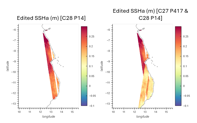
Bias anomaly for a pass parallel to the coast