Processing

This section describes the processing of the SWOT L3 KaRIn (L3_LR_SSH) product. This product contains the KaRIn measurements as well as the Nadir measurements (only in Expert and Basic products): KaRIn and Nadir instruments are blended into a single image.

Note that a presentation dedicated to the processing named “SWOT Level-3 Overview and link with L2 products”, from Dibarboure et al., have been presented at the SWOT Science Team in June 2024. The processing methodology for SWOT level 3 products is outlined in a paper by Dibarboure et al. (2024).

Processing method

The following figure provides an overview of the system for the generation of the SWOT L3 KaRIn ocean product. The Nadir component follows the same processing as the other altimeters as described in Pujol et al., 2023, and the L3 KaRIn processing sequence is given. The resultant L3 KaRIn ocean product contain both KaRIn and Nadir measurements.

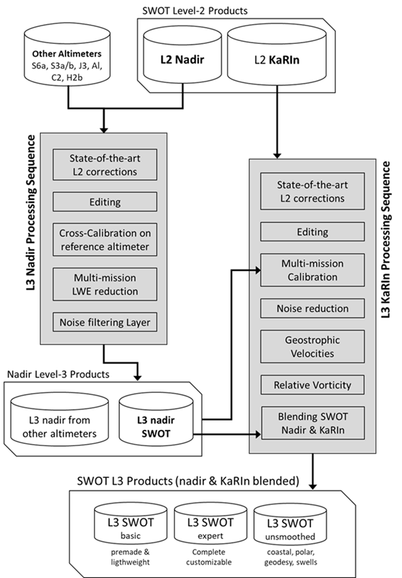
DUACS and SWOT L3 KaRIn and Nadir system processing

Input data

The input data used to compute the SWOT L3 KaRIn ocean product is the SWOT L2_LR_SSH, defined with a 2x2km or 250x250m spatial posting rate and distributed by the CDS-AVISO (https://doi.org/10.24400/527896/a01-2023.015). The version of these products evolves with time. The standard table lists the L2_LR_SSH product versions used in the L3_LR_SSH production.

250m swath reconstruction

The L2 LR 250m product presents the data into separated ‘left’ and ‘right’ swaths, with possibly missing lines in the swath grid definition. A specific acquisition aims to consolidate the product into a unified format compatible with other the LR datasets defined on a reference grid (no missing lines, no left/right separation).

The acquisition and preprocessing of the L2 LR 250m product performs several crucial steps to achieve this unification:

Swath Merging

The unsmoothed products contain distinct data groups for the left and right instrument swaths. A core function merges these two sections into a single, continuous 2D array. This involves flipping the left swath and concatenating it with the right. A 39-pixel gap is inserted at the center to represent the nadir gap, ensuring a continuous cross-track dataset

Time Synchronization

The script reads and validates the time vectors from both swaths. It then computes a single, unified time vector for each measurement line, typically by averaging the left and right timestamps.

Data Masking

Invalid measurements are meticulously filtered out. A Boolean mask is generated based on valid latitude and time values, ensuring that only robust data points are processed and stored.

Variable Reading

Data loading is primarily handled by a variable reader. This function iterates through a list of specified product files and reads the designated variables. The valid data mask is consistently applied to all variables, guaranteeing uniform dimensions across the dataset.

Geolocation Interpolation

For longitude and latitude variables, a dedicated function interpolates any gaps in the geolocation data. This step is vital for constructing a complete and continuous swath.

Generating Supplemental Variables

To maintain compatibility with standard LR products, the script can generate variables not present in the original unsmoothed files

• cross_track_distance: Calculated by a function based on a predefined instrument geometry.

• valid_location_flag: Generated by a function to indicate whether the geolocation at each pixel is original or was filled via interpolation.

Metadata Extraction

Essential metadata, such as cycle_number and pass_number, are extracted directly from the product filenames using a regular expression pattern.

Up-to-date standards

The measurements are then updated with the standards as follows

V3.0V2.0 and V2.0.1V1.0.2V1.0

Standard reference	PGC0 before 10/01/2024 PIC0/PIC2/PID0 after
Orbit	POE-F
Ionospheric	GIM model computed from vertical Total Electron Content maps (Chou et al. 2023) rescaled on the orbit altitude with IRI95 model (https://irimodel.org/)
Wet troposphere	Model computed from ECMWF Gaussian grids
Sea State Bias	Non-parametric SSB from AltiKa GDR-F (Tran 2019) with corrected SWH MFWAM model field
Mean Profile/ Mean Sea Surface	MSS CNES_CLS_2025 (beta release, Charayron et al. 2025)
Mean Dynamic Topography	MDT CNES_CLS_2022 (Jousset and Mulet 2020, Jousset et al. 2022) with a -5cm offset
Dry troposphere	Model computed from ECMWF Gaussian grids (new S1 and S2 atmospheric tides are applied)
DAC	DAC v4.0: TUGO forced with ECMWF pressure and wing fields (S1 and S2 were excluded) + inverse barometer computed from rectangular grids
Ocean tide	FES2022: (Lyard et al. 2023, Loren Carrère et al. 2023) (https://doi.org/10.24400/527896/a01-2024.004) from unstructured grid when available and completed with cartesian grid
Internal tide	(Zaron E. et Elipot S. 2024) ( blend of HRET14 & HRET8.1, tidal frequencies: M2, K1, S2, O1, N2)
Pole tide	(Desai, Wahr, et Beckley 2015)& Mean Pole Location
Solid earth tide	Elastic response to tidal potential (Cartwright et Edden 1973, Cartwright et Tayler 1971)
Loading tide	FES2022: (Lyard et al. 2023, Loren Carrère et al. 2023)

Cross-calibration

The correction is computed with the XCAL algorithm. The reference for the XCAL algorithm is Dibarboure et al., June 2022, SWOT Science Team meeting, SWOT simulated Level-2 and Level-3 data-driven calibration and Dibarboure et al., Sep 2023, SWOT Science Team meeting, Crossover Calibration Status and Examples.

The Level-3 calibration correction aims to reduce systematic errors in KaRIn and ensure its measurements are consistent with L3 products from other altimeter missions. Therefore, data from operational nadir altimeters are used in the KaRIn calibration process. KaRIn systematic errors are first estimated over ocean areas using pre-selected KaRIn measurements. The residuals, relative to multi-mission nadir data, are decomposed into roll errors and phase-screen errors. The resulting calibration correction is then interpolated over invalid measurement areas, including holes over ocean, continents and polar areas. This calibration is estimated using LR 2x2km upstream data.

The methodology has been refined through successive versions of L3 products.

In the L3 V1.0 version, the calibration has been improved with an updated phase screen correction with two components (varying with beta angle and in-orbit position) and an improved interpolation method for short segments

In the v2.0 version, the calibration has been improved with the aim of reducing the leakage of the ocean dynamic signal and taking into account the improvements made to the data selection processing:

• A large part of the data selection is newly applied before calibration

• Data eclipse transition segments are used in the calibration

• Fewer degrees of freedom are used

• L3 pseudo phase screen corrections remain unchanged w.r.t v1.0.2

In the V3.0 version, the calibration has been improved with a better estimation of the roll errors by adding harmonics on the day frequency; the use of an optimal interpolation methodology to estimate the roll correction in areas where direct estimation is not possible; and update of the static phase screen component for the PID product version.

The correction applied on the 250x250m product is an interpolation of the solution computed using 2x2km data.

Editing

The editing process mainly consists in applying the flags that are in the L2_LR_SSH input files. The variables taken into account are:

• ancillary_surface_classification_flag (to keep only ocean data)

• ssha_KaRIn_2_qual (L2 product flags)

• ssh_KaRIn_uncert (measurement uncertainty)

• distance_to_coast (for the coastal flag)

• cross_track_distance (distance from the nadir)

• Ice_concentration (for the polar flag)

• sig0_karin_2 (for the sea-ice classification of the Unsmoothed product)

• rain_rate_rf (for the rain flag)

From the L3_LR_SSH v1.0, a flag expert was created. Its content has been refined throughout the successive versions of L3 products. The following table gives the different flag values available for each version.

V3.0V2.0 and V2.0.1V1.0

• Flag #102: No SSHa values available

• Flag #101: Pixels over land

• Flag #100: Edges of swath. Only values between 10 to 60 km to the nadir are considered as valid data

• Flag #70: Pixels impacted by spacecraft events

• Flag #50: Abnormally high SSHA values

• Flag #25: Rain Cells

• Flag #30: SSHA pixels out of the expected statistical distribution

• Flag #20: Suspected sea-ice pixels (high probability)

• Flag #19: Suspected sea-ice pixels (medium probability) [Unsmoothed only]

• Flag #18: Suspected ocean pixels (medium probability) [Unsmoothed only]

• Flag #10: Suspected coastal pixels

• Flag #5: SSHA pixels out of the local distribution.

• Flag #3: Eclipses

• Flag #0: Valid data

More details about each flag are available in Dibarboure et al (2024). The following figures show some cases of use of the flag expert. For most studies, we recommend keeping only flag #0 to flag #3.

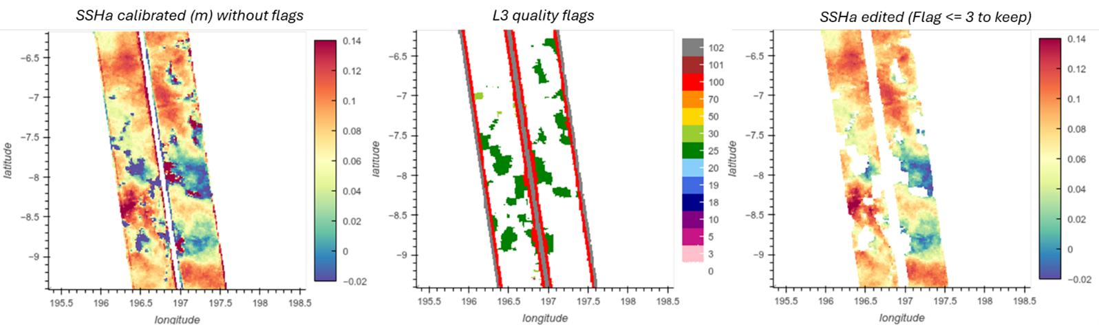
Example of editing of the rain cells (C19 P556). Keeping flags #0 to #3 (v2.0.1 and later versions) is recommended

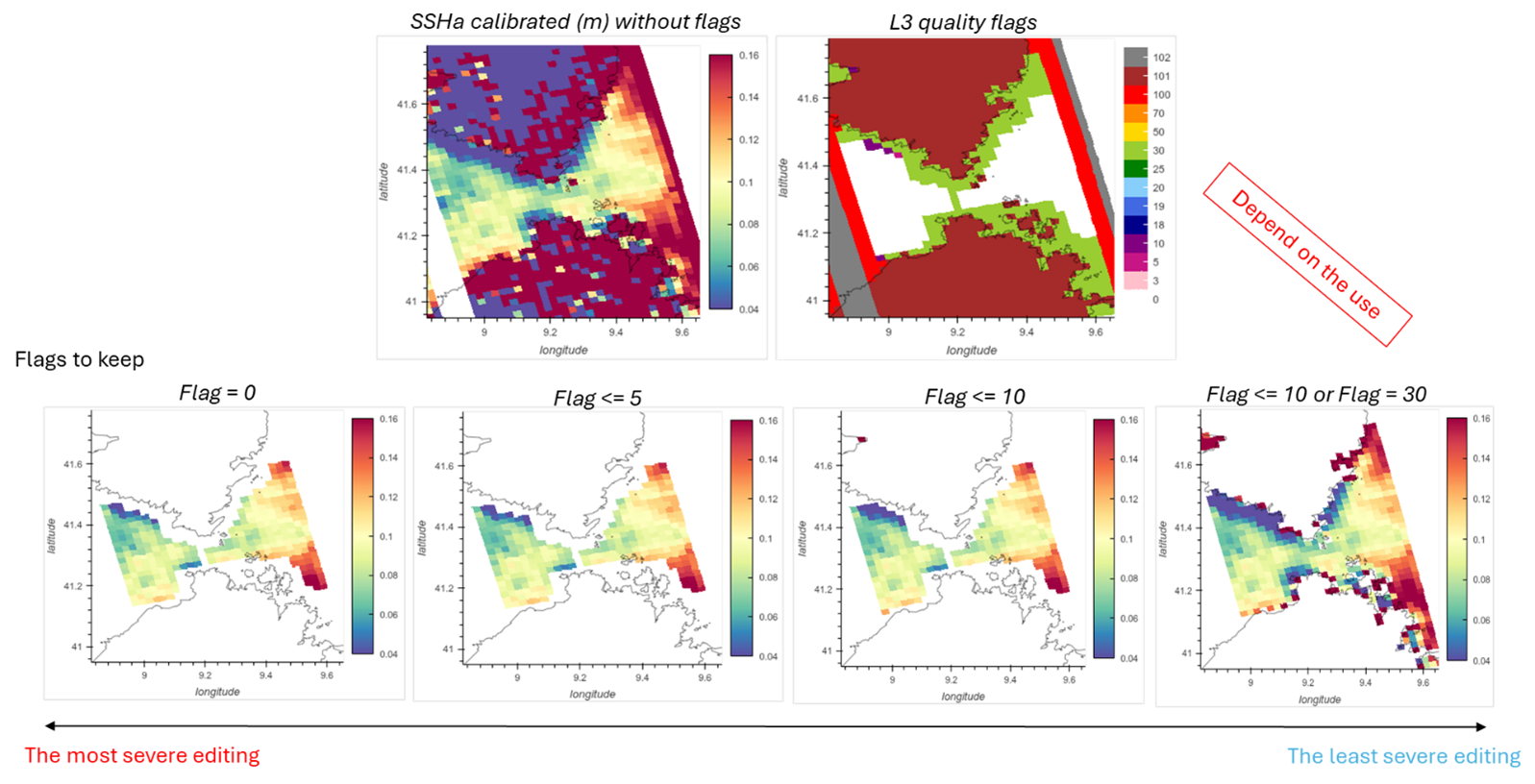
Figure 4: Example of editing of coastlines (C19 P542) in v3.0

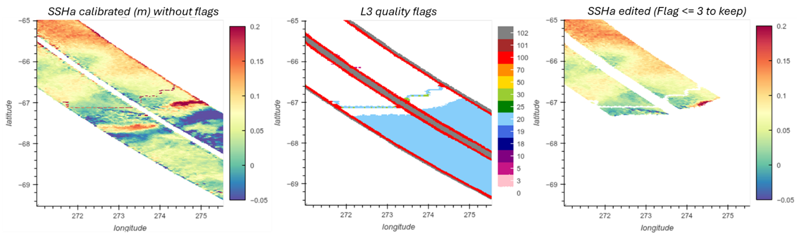
Example of editing of polar (C19 P552) areas in v3.0

Filtering

Despite its unprecedented precision, SWOT’s Ka-band Radar Interferometer (KaRIn) still exhibits a substantial amount of random noise. A filtering method is then applied, it is described in Treboutte et al., 2023. It consists of a Neural Network which is based on a U-Net architecture and is trained and tested with simulated data from the North Atlantic.

The following table presents the denoising differences between the different versions of the L3_LR_SSH products

	Version 0.3	Version 1.0 to 2.0.1	Version 3.0
Training dataset	Based on the eNATL60 ocean model without tides Noise generated by the SWOT simulator	Based on the eNATL60 ocean model with tides. Correlated Noise generated by style transfer to be as realistic as possible	Based on the eNATL60 ocean model with tides. Realistic editing from L3 real swaths is applied on simulated swaths. No style-transfer
Use of the [Gomez et al, 2020] algorithm	Yes	No	No

More details about the training dataset are available in Dibarboure et al. (2024).

The following figure shows the impact of the filtering in the resultant current and the vorticity

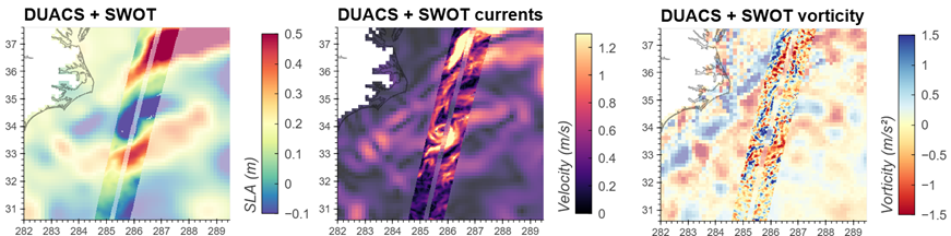
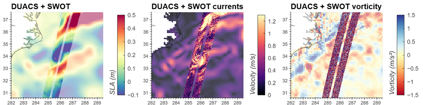
Sea Level Anomalies of DUACS and SWOT L3 v3.0 measurements (left), deduced current (middle) and vorticity (right) with the denoising applied (top) and without (bottom)

SSHA derivatives and geostrophic currents estimation

An estimation of the geostrophic currents is proposed in L3 KaRIn products. The methodology used to compute the anomaly of the currant is presented in the following table. The mean current is issued from the MDT field (Jousset et al. 2025)

Version 0.3	Version 1.0 to 2.0.1	Version 3.0
2-points stencil methodology from “denoised” SSHA. in along and across swath direction. The current is then interpolated on Northward and Eastward direction	6-points stencil methodology from “denoised” SSHA. in along and across swath direction. The current is then interpolated on Northward and Eastward direction. An estimation of the SSH gradients from unfiltered (raw) SSHA measurements is also proposed using the same methodology	2D spline fitting for “denoised” SSHA (Tranchant et al. 2025) An estimation of the SSH gradients from “unfiltered” (raw) SSHA measurements is also proposed using the same methodology

Know limitations

The SSH measured by KaRIn is not just from mesoscale but also a synoptic view of unbalanced motions and barotropic residuals. Denoising/filtering processing applied may not allow to accurately extract the balanced motion. Specifically, geostrophy assumption might simply no longer be relevant for the smallest scales observed by KaRIn