Download notebook.

Copyright CNES

Read and plot a SWOT-HR Raster products

In this notebook, we show how to read the SWOT-HR raster 100m and 250m netcdf products with xarray and how to represent a variable on a map with cartopy.

Libraries

Please note that apart from the libraries listed in the cell below, you need to install the h5netcdf library (conda install -c conda-forge h5netcdf). This will be used by th xarray.open_dataset function to read the netcdf files.

import xarray as xr
import rioxarray
from pyproj import CRS
import os
import numpy as np
import matplotlib.pyplot as plt
%matplotlib inline

1. Read a SWOT-HR Raster netcdf product with xarray

dir_swot = "../docs/data/swot/"
file_swot_raster100 = os.path.join(
    dir_swot,
    "SWOT_L2_HR_Raster_100m",
    "SWOT_L2_HR_Raster_100m_UTM22N_N_x_x_x_015_033_082F_20240509T115817_20240509T115835_PIC0_01_extract.nc",
)
# read data with xarray
xr_swot_raster100 = xr.open_dataset(file_swot_raster100)
# force xarray to acknowledge the CRS
xr_swot_raster100.rio.set_crs(CRS.from_user_input(xr_swot_raster100.crs.projected_crs_name).to_epsg(), inplace=True)

xr_swot_raster100

<xarray.Dataset>
Dimensions:                  (y: 75, x: 59)
Coordinates:
  * x                        (x) float64 2.712e+05 2.713e+05 ... 2.77e+05
  * y                        (y) float64 5.558e+05 5.559e+05 ... 5.632e+05
Data variables: (12/39)
    cross_track              (y, x) float32 ...
    crs                      object ...
    dark_frac                (y, x) float32 ...
    geoid                    (y, x) float32 ...
    height_cor_xover         (y, x) float32 ...
    ice_clim_flag            (y, x) float32 ...
    ...                       ...
    water_frac               (y, x) float32 ...
    water_frac_uncert        (y, x) float32 ...
    wse                      (y, x) float32 ...
    wse_qual                 (y, x) float32 ...
    wse_qual_bitwise         (y, x) float64 ...
    wse_uncert               (y, x) float32 ...
Attributes: (12/50)
    Conventions:                   CF-1.7
    title:                         Level 2 KaRIn High Rate Raster Data Product
    source:                        Ka-band radar interferometer
    history:                       Wed Jun  5 21:08:21 2024: ncks -d x,271195...
    platform:                      SWOT
    references:                    V1.2.1
    ...                            ...
    x_max:                         315500.0
    y_min:                         497300.0
    y_max:                         643000.0
    institution:                   CNES
    product_version:               01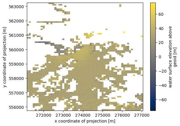
    NCO:                           netCDF Operators version 5.0.6 (Homepage =...

xarray.Dataset

• Dimensions:
  • y: 75
  • x: 59
• Coordinates: (2)
  • x
    (x)
    float64
    2.712e+05 2.713e+05 ... 2.77e+05

    long_name :

    x coordinate of projection

    standard_name :

    projection_x_coordinate

    units :

    m

    valid_min :

    -10000000.0

    valid_max :

    10000000.0

    comment :

    UTM easting coordinate of the pixel.

    array([271200., 271300., 271400., 271500., 271600., 271700., 271800., 271900.,
           272000., 272100., 272200., 272300., 272400., 272500., 272600., 272700.,
           272800., 272900., 273000., 273100., 273200., 273300., 273400., 273500.,
           273600., 273700., 273800., 273900., 274000., 274100., 274200., 274300.,
           274400., 274500., 274600., 274700., 274800., 274900., 275000., 275100.,
           275200., 275300., 275400., 275500., 275600., 275700., 275800., 275900.,
           276000., 276100., 276200., 276300., 276400., 276500., 276600., 276700.,
           276800., 276900., 277000.])

  • y
    (y)
    float64
    5.558e+05 5.559e+05 ... 5.632e+05

    long_name :

    y coordinate of projection

    standard_name :

    projection_y_coordinate

    units :

    m

    valid_min :

    -20000000.0

    valid_max :

    20000000.0

    comment :

    UTM northing coordinate of the pixel.

    array([555800., 555900., 556000., 556100., 556200., 556300., 556400., 556500.,
           556600., 556700., 556800., 556900., 557000., 557100., 557200., 557300.,
           557400., 557500., 557600., 557700., 557800., 557900., 558000., 558100.,
           558200., 558300., 558400., 558500., 558600., 558700., 558800., 558900.,
           559000., 559100., 559200., 559300., 559400., 559500., 559600., 559700.,
           559800., 559900., 560000., 560100., 560200., 560300., 560400., 560500.,
           560600., 560700., 560800., 560900., 561000., 561100., 561200., 561300.,
           561400., 561500., 561600., 561700., 561800., 561900., 562000., 562100.,
           562200., 562300., 562400., 562500., 562600., 562700., 562800., 562900.,
           563000., 563100., 563200.])

• Data variables: (39)
  • cross_track
    (y, x)
    float32
    ...

    long_name :

    approximate cross-track location

    grid_mapping :

    crs

    units :

    m

    valid_min :

    -75000.0

    valid_max :

    75000.0

    comment :

    Approximate cross-track location of the pixel.

    [4425 values with dtype=float32]

  • crs
    ()
    object
    ...

    long_name :

    CRS Definition

    grid_mapping_name :

    transverse_mercator

    projected_crs_name :

    WGS 84 / UTM zone 22N

    geographic_crs_name :

    WGS 84

    reference_ellipsoid_name :

    WGS 84

    horizontal_datum_name :

    WGS_1984

    prime_meridian_name :

    Greenwich

    false_easting :

    500000.0

    false_northing :

    0.0

    longitude_of_central_meridian :

    -51.0

    longitude_of_prime_meridian :

    0.0

    latitude_of_projection_origin :

    0.0

    scale_factor_at_central_meridian :

    0.9996

    semi_major_axis :

    6378137.0

    inverse_flattening :

    298.257223563

    crs_wkt :

    PROJCS["WGS 84 / UTM zone 22N",GEOGCS["WGS 84",DATUM["WGS_1984",SPHEROID["WGS 84",6378137,298.257223563,AUTHORITY["EPSG","7030"]],AUTHORITY["EPSG","6326"]],PRIMEM["Greenwich",0,AUTHORITY["EPSG","8901"]],UNIT["degree",0.0174532925199433,AUTHORITY["EPSG","9122"]],AUTHORITY["EPSG","4326"]],PROJECTION["Transverse_Mercator"],PARAMETER["latitude_of_origin",0],PARAMETER["central_meridian",-51],PARAMETER["scale_factor",0.9996],PARAMETER["false_easting",500000],PARAMETER["false_northing",0],UNIT["metre",1,AUTHORITY["EPSG","9001"]],AXIS["Easting",EAST],AXIS["Northing",NORTH],AUTHORITY["EPSG","32622"]]

    spatial_ref :

    PROJCS["WGS 84 / UTM zone 22N",GEOGCS["WGS 84",DATUM["WGS_1984",SPHEROID["WGS 84",6378137,298.257223563,AUTHORITY["EPSG","7030"]],AUTHORITY["EPSG","6326"]],PRIMEM["Greenwich",0,AUTHORITY["EPSG","8901"]],UNIT["degree",0.0174532925199433,AUTHORITY["EPSG","9122"]],AUTHORITY["EPSG","4326"]],PROJECTION["Transverse_Mercator"],PARAMETER["latitude_of_origin",0],PARAMETER["central_meridian",-51],PARAMETER["scale_factor",0.9996],PARAMETER["false_easting",500000],PARAMETER["false_northing",0],UNIT["metre",1,AUTHORITY["EPSG","9001"]],AXIS["Easting",EAST],AXIS["Northing",NORTH],AUTHORITY["EPSG","32622"]]

    comment :

    UTM zone coordinate reference system.

    [1 values with dtype=object]

  • dark_frac
    (y, x)
    float32
    ...

    long_name :

    fractional area of dark water

    grid_mapping :

    crs

    units :

    l

    valid_min :

    -1000.0

    valid_max :

    10000.0

    comment :

    Fraction of pixel water surface area covered by dark water.

    [4425 values with dtype=float32]

  • geoid
    (y, x)
    float32
    ...

    long_name :

    geoid height

    standard_name :

    geoid_height_above_reference_ellipsoid

    source :

    EGM2008 (Pavlis et al., 2012)

    grid_mapping :

    crs

    units :

    m

    valid_min :

    -150.0

    valid_max :

    150.0

    comment :

    Geoid height above the reference ellipsoid with a correction to refer the value to the mean tide system, i.e. includes the permanent tide (zero frequency).

    [4425 values with dtype=float32]

  • height_cor_xover
    (y, x)
    float32
    ...

    long_name :

    height correction from KaRIn crossovers

    grid_mapping :

    crs

    units :

    m

    valid_min :

    -10.0

    valid_max :

    10.0

    comment :

    Height correction from KaRIn crossover calibration. The correction is applied before geolocation but reported as an equivalent height correction.

    [4425 values with dtype=float32]

  • ice_clim_flag
    (y, x)
    float32
    ...

    long_name :

    climatological ice cover flag

    standard_name :

    status_flag

    source :

    UNC

    grid_mapping :

    crs

    flag_meanings :

    no_ice_cover uncertain_ice_cover full_ice_cover

    flag_values :

    [0 1 2]

    valid_min :

    0

    valid_max :

    2

    comment :

    Climatological ice cover flag indicating whether the pixel is ice-covered on the day of the observation based on external climatological information (not the SWOT measurement). Values of 0, 1, and 2 indicate that the pixel is likely not ice covered, may or may not be partially or fully ice covered, and likely fully ice covered, respectively.

    [4425 values with dtype=float32]

  • ice_dyn_flag
    (y, x)
    float32
    ...

    long_name :

    dynamic ice cover flag

    standard_name :

    status_flag

    source :

    UNC

    grid_mapping :

    crs

    flag_meanings :

    no_ice_cover partial_ice_cover full_ice_cover

    flag_values :

    [0 1 2]

    valid_min :

    0

    valid_max :

    2

    comment :

    Dynamic ice cover flag indicating whether the surface is ice-covered on the day of the observation based on analysis of external satellite optical data. Values of 0, 1, and 2 indicate that the pixel is not ice covered, partially ice covered, and fully ice covered, respectively.

    [4425 values with dtype=float32]

  • illumination_time
    (y, x)
    datetime64[ns]
    ...

    long_name :

    time of illumination of each pixel (UTC)

    standard_name :

    time

    tai_utc_difference :

    37.0

    leap_second :

    0000-00-00T00:00:00Z

    comment :

    Time of measurement in seconds in the UTC time scale since 1 Jan 2000 00:00:00 UTC. [tai_utc_difference] is the difference between TAI and UTC reference time (seconds) for the first measurement of the data set. If a leap second occurs within the data set, the attribute leap_second is set to the UTC time at which the leap second occurs.

    [4425 values with dtype=datetime64[ns]]

  • illumination_time_tai
    (y, x)
    datetime64[ns]
    ...

    long_name :

    time of illumination of each pixel (TAI)

    standard_name :

    time

    comment :

    Time of measurement in seconds in the TAI time scale since 1 Jan 2000 00:00:00 TAI. This time scale contains no leap seconds. The difference (in seconds) with time in UTC is given by the attribute [illumination_time:tai_utc_difference].

    [4425 values with dtype=datetime64[ns]]

  • inc
    (y, x)
    float32
    ...

    long_name :

    incidence angle

    grid_mapping :

    crs

    units :

    degrees

    valid_min :

    0.0

    valid_max :

    90.0

    comment :

    Incidence angle.

    [4425 values with dtype=float32]

  • iono_cor_gim_ka
    (y, x)
    float32
    ...

    long_name :

    ionosphere vertical correction

    source :

    Global Ionosphere Maps

    institution :

    JPL

    grid_mapping :

    crs

    units :

    m

    valid_min :

    -0.5

    valid_max :

    0.0

    comment :

    Equivalent vertical correction due to ionosphere delay. The reported water surface elevation, latitude and longitude are computed after adding negative media corrections to uncorrected range along slant-range paths, accounting for the differential delay between the two KaRIn antennas. The equivalent vertical correction is computed by applying obliquity factors to the slant-path correction. Adding the reported correction to the reported water surface elevation results in the uncorrected pixel height.

    [4425 values with dtype=float32]

  • latitude
    (y, x)
    float64
    ...

    long_name :

    latitude (positive N, negative S)

    standard_name :

    latitude

    grid_mapping :

    crs

    units :

    degrees_north

    valid_min :

    -80.0

    valid_max :

    80.0

    comment :

    Geodetic latitude [-80,80] (degrees north of equator) of the pixel.

    [4425 values with dtype=float64]

  • layover_impact
    (y, x)
    float32
    ...

    long_name :

    layover impact

    grid_mapping :

    crs

    units :

    m

    valid_min :

    -999999.0

    valid_max :

    999999.0

    comment :

    Estimate of the water surface elevation error caused by layover.

    [4425 values with dtype=float32]

  • load_tide_fes
    (y, x)
    float32
    ...

    long_name :

    geocentric load tide height (FES)

    source :

    FES2014b (Carrere et al., 2016)

    institution :

    LEGOS/CNES

    grid_mapping :

    crs

    units :

    m

    valid_min :

    -0.2

    valid_max :

    0.2

    comment :

    Geocentric load tide height. The effect of the ocean tide loading of the Earth’s crust.

    [4425 values with dtype=float32]

  • load_tide_got
    (y, x)
    float32
    ...

    long_name :

    geocentric load tide height (GOT)

    source :

    GOT4.10c (Ray, 2013)

    institution :

    GSFC

    grid_mapping :

    crs

    units :

    m

    valid_min :

    -0.2

    valid_max :

    0.2

    comment :

    Geocentric load tide height. The effect of the ocean tide loading of the Earth’s crust. This value is reported for reference but is not applied to the reported height.

    [4425 values with dtype=float32]

  • longitude
    (y, x)
    float64
    ...

    long_name :

    longitude (degrees East)

    standard_name :

    longitude

    grid_mapping :

    crs

    units :

    degrees_east

    valid_min :

    -180.0

    valid_max :

    180.0

    comment :

    Geodetic longitude [-180,180) (east of the Greenwich meridian) of the pixel.

    [4425 values with dtype=float64]

  • model_dry_tropo_cor
    (y, x)
    float32
    ...

    long_name :

    dry troposphere vertical correction

    source :

    European Centre for Medium-Range Weather Forecasts

    institution :

    ECMWF

    grid_mapping :

    crs

    units :

    m

    valid_min :

    -3.0

    valid_max :

    -1.5

    comment :

    Equivalent vertical correction due to dry troposphere delay. The reported water surface elevation, latitude and longitude are computed after adding negative media corrections to uncorrected range along slant-range paths, accounting for the differential delay between the two KaRIn antennas. The equivalent vertical correction is computed by applying obliquity factors to the slant-path correction. Adding the reported correction to the reported water surface elevation results in the uncorrected pixel height.

    [4425 values with dtype=float32]

  • model_wet_tropo_cor
    (y, x)
    float32
    ...

    long_name :

    wet troposphere vertical correction

    source :

    European Centre for Medium-Range Weather Forecasts

    institution :

    ECMWF

    grid_mapping :

    crs

    units :

    m

    valid_min :

    -1.0

    valid_max :

    0.0

    comment :

    Equivalent vertical correction due to wet troposphere delay. The reported water surface elevation, latitude and longitude are computed after adding negative media corrections to uncorrected range along slant-range paths, accounting for the differential delay between the two KaRIn antennas. The equivalent vertical correction is computed by applying obliquity factors to the slant-path correction. Adding the reported correction to the reported water surface elevation results in the uncorrected pixel height.

    [4425 values with dtype=float32]

  • n_other_pix
    (y, x)
    float64
    ...

    long_name :

    number of other pixels

    grid_mapping :

    crs

    units :

    l

    valid_min :

    0

    valid_max :

    999999

    comment :

    Number of pixel cloud samples used in aggregation of quantities not related to water surface elevation, water surface area, water fraction or sigma0.

    [4425 values with dtype=float64]

  • n_sig0_pix
    (y, x)
    float64
    ...

    long_name :

    number of sigma0 pixels

    grid_mapping :

    crs

    units :

    l

    valid_min :

    0

    valid_max :

    999999

    comment :

    Number of pixel cloud samples used in sigma0 aggregation.

    [4425 values with dtype=float64]

  • n_water_area_pix
    (y, x)
    float64
    ...

    long_name :

    number of water surface area pixels

    grid_mapping :

    crs

    units :

    l

    valid_min :

    0

    valid_max :

    999999

    comment :

    Number of pixel cloud samples used in water surface area and water fraction aggregation.

    [4425 values with dtype=float64]

  • n_wse_pix
    (y, x)
    float64
    ...

    long_name :

    number of water surface elevation pixels

    grid_mapping :

    crs

    units :

    l

    valid_min :

    0

    valid_max :

    999999

    comment :

    Number of pixel cloud samples used in water surface elevation aggregation.

    [4425 values with dtype=float64]

  • pole_tide
    (y, x)
    float32
    ...

    long_name :

    geocentric pole tide height

    source :

    Wahr (1985) and Desai et al. (2015)

    grid_mapping :

    crs

    units :

    m

    valid_min :

    -0.2

    valid_max :

    0.2

    comment :

    Geocentric pole tide height. The total of the contribution from the solid-Earth (body) pole tide height and the load pole tide height (i.e., the effect of the ocean pole tide loading of the Earth’s crust).

    [4425 values with dtype=float32]

  • sig0
    (y, x)
    float32
    ...

    long_name :

    sigma0

    grid_mapping :

    crs

    units :

    1

    quality_flag :

    sig0_qual

    valid_min :

    -999999.0

    valid_max :

    999999.0

    comment :

    Normalized radar cross section (sigma0) in real, linear units (not decibels). The value may be negative due to noise subtraction.

    [4425 values with dtype=float32]

  • sig0_cor_atmos_model
    (y, x)
    float32
    ...

    long_name :

    two-way atmospheric correction to sigma0 from model

    source :

    European Centre for Medium-Range Weather Forecasts

    institution :

    ECMWF

    grid_mapping :

    crs

    units :

    1

    valid_min :

    1.0

    valid_max :

    10.0

    comment :

    Atmospheric correction to sigma0 from weather model data as a linear power multiplier (not decibels). sig0_cor_atmos_model is already applied in computing sig0.

    [4425 values with dtype=float32]

  • sig0_qual
    (y, x)
    float32
    ...

    long_name :

    summary quality indicator for the sigma0

    standard_name :

    status_flag

    grid_mapping :

    crs

    flag_meanings :

    good suspect degraded bad

    flag_values :

    [0 1 2 3]

    valid_min :

    0

    valid_max :

    3

    comment :

    Summary quality indicator for the sigma0 quantities. A value of 0 indicates a nominal measurement, 1 indicates a suspect measurement, 2 indicates a degraded measurement, and 3 indicates a bad measurement.

    [4425 values with dtype=float32]

  • sig0_qual_bitwise
    (y, x)
    float64
    ...

    long_name :

    bitwise quality indicator for the sigma0

    standard_name :

    status_flag

    grid_mapping :

    crs

    flag_meanings :

    sig0_qual_suspect classification_qual_suspect geolocation_qual_suspect large_uncert_suspect bright_land low_coherence_water_suspect few_pixels far_range_suspect near_range_suspect sig0_qual_degraded classification_qual_degraded geolocation_qual_degraded value_bad outside_data_window no_pixels outside_scene_bounds inner_swath missing_karin_data

    flag_masks :

    [ 1 2 4 32 128 256 4096 8192 16384 131072 262144 524288 16777216 67108864 268435456 536870912 1073741824 2147483648]

    valid_min :

    0

    valid_max :

    4111364519

    comment :

    Bitwise quality indicator for the sigma0 quantities. If this word is interpreted as an unsigned integer, a value of 0 indicates good data, positive values less than 32768 represent suspect data, values greater than or equal to 32768 but less than 8388608 represent degraded data, and values greater than or equal to 8388608 represent bad data.

    [4425 values with dtype=float64]

  • sig0_uncert
    (y, x)
    float32
    ...

    long_name :

    uncertainty in sigma0

    grid_mapping :

    crs

    units :

    1

    valid_min :

    -999999.0

    valid_max :

    999999.0

    comment :

    1-sigma uncertainty in sigma0. The value is provided in linear units. This value is a one-sigma additive (not multiplicative) uncertainty term, which can be added to or subtracted from sigma0.

    [4425 values with dtype=float32]

  • solid_earth_tide
    (y, x)
    float32
    ...

    long_name :

    solid Earth tide height

    source :

    Cartwright and Taylor (1971) and Cartwright and Edden (1973)

    grid_mapping :

    crs

    units :

    m

    valid_min :

    -1.0

    valid_max :

    1.0

    comment :

    Solid-Earth (body) tide height. The zero-frequency permanent tide component is not included.

    [4425 values with dtype=float32]

  • water_area
    (y, x)
    float32
    ...

    long_name :

    water surface area

    grid_mapping :

    crs

    units :

    m^2

    quality_flag :

    water_area_qual

    valid_min :

    -2000000.0

    valid_max :

    2000000000.0

    comment :

    Surface area of the water pixels.

    [4425 values with dtype=float32]

  • water_area_qual
    (y, x)
    float32
    ...

    long_name :

    summary quality indicator for the water surface area

    standard_name :

    status_flag

    grid_mapping :

    crs

    flag_meanings :

    good suspect degraded bad

    flag_values :

    [0 1 2 3]

    valid_min :

    0

    valid_max :

    3

    comment :

    Summary quality indicator for the water surface area and water fraction quantities. A value of 0 indicates a nominal measurement, 1 indicates a suspect measurement, 2 indicates a degraded measurement, and 3 indicates a bad measurement.

    [4425 values with dtype=float32]

  • water_area_qual_bitwise
    (y, x)
    float64
    ...

    long_name :

    bitwise quality indicator for the water surface area

    standard_name :

    status_flag

    grid_mapping :

    crs

    flag_meanings :

    classification_qual_suspect geolocation_qual_suspect water_fraction_suspect large_uncert_suspect bright_land low_coherence_water_suspect few_pixels far_range_suspect near_range_suspect classification_qual_degraded geolocation_qual_degraded value_bad outside_data_window no_pixels outside_scene_bounds inner_swath missing_karin_data

    flag_masks :

    [ 2 4 8 32 128 256 4096 8192 16384 262144 524288 16777216 67108864 268435456 536870912 1073741824 2147483648]

    valid_min :

    0

    valid_max :

    4111233454

    comment :

    Bitwise quality indicator for the water surface area and water fraction quantities. If this word is interpreted as an unsigned integer, a value of 0 indicates good data, positive values less than 32768 represent suspect data, values greater than or equal to 32768 but less than 8388608 represent degraded data, and values greater than or equal to 8388608 represent bad data.

    [4425 values with dtype=float64]

  • water_area_uncert
    (y, x)
    float32
    ...

    long_name :

    uncertainty in the water surface area

    grid_mapping :

    crs

    units :

    m^2

    valid_min :

    0.0

    valid_max :

    2000000000.0

    comment :

    1-sigma uncertainty in the water surface area.

    [4425 values with dtype=float32]

  • water_frac
    (y, x)
    float32
    ...

    long_name :

    water fraction

    grid_mapping :

    crs

    units :

    1

    quality_flag :

    water_area_qual

    valid_min :

    -1000.0

    valid_max :

    10000.0

    comment :

    Fraction of the pixel that is water.

    [4425 values with dtype=float32]

  • water_frac_uncert
    (y, x)
    float32
    ...

    long_name :

    uncertainty in the water fraction

    grid_mapping :

    crs

    units :

    1

    valid_min :

    0.0

    valid_max :

    999999.0

    comment :

    1-sigma uncertainty in the water fraction.

    [4425 values with dtype=float32]

  • wse
    (y, x)
    float32
    ...

    long_name :

    water surface elevation above geoid

    grid_mapping :

    crs

    units :

    m

    quality_flag :

    wse_qual

    valid_min :

    -1500.0

    valid_max :

    15000.0

    comment :

    Water surface elevation of the pixel above the geoid and after using models to subtract the effects of tides (solid_earth_tide, load_tide_fes, pole_tide).

    [4425 values with dtype=float32]

  • wse_qual
    (y, x)
    float32
    ...

    long_name :

    summary quality indicator for the water surface elevation

    standard_name :

    status_flag

    grid_mapping :

    crs

    flag_meanings :

    good suspect degraded bad

    flag_values :

    [0 1 2 3]

    valid_min :

    0

    valid_max :

    3

    comment :

    Summary quality indicator for the water surface elevation quantities. A value of 0 indicates a nominal measurement, 1 indicates a suspect measurement, 2 indicates a degraded measurement, and 3 indicates a bad measurement.

    [4425 values with dtype=float32]

  • wse_qual_bitwise
    (y, x)
    float64
    ...

    long_name :

    bitwise quality indicator for the water surface elevation

    standard_name :

    status_flag

    grid_mapping :

    crs

    flag_meanings :

    classification_qual_suspect geolocation_qual_suspect large_uncert_suspect bright_land few_pixels far_range_suspect near_range_suspect classification_qual_degraded geolocation_qual_degraded dark_water_degraded low_coherence_water_degraded value_bad outside_data_window no_pixels outside_scene_bounds inner_swath missing_karin_data

    flag_masks :

    [ 2 4 32 128 4096 8192 16384 262144 524288 1048576 2097152 16777216 67108864 268435456 536870912 1073741824 2147483648]

    valid_min :

    0

    valid_max :

    4114378918

    comment :

    Bitwise quality indicator for the water surface elevation quantities. If this word is interpreted as an unsigned integer, a value of 0 indicates good data, positive values less than 32768 represent suspect data, values greater than or equal to 32768 but less than 8388608 represent degraded data, and values greater than or equal to 8388608 represent bad data.

    [4425 values with dtype=float64]

  • wse_uncert
    (y, x)
    float32
    ...

    long_name :

    uncertainty in the water surface elevation

    grid_mapping :

    crs

    units :

    m

    valid_min :

    0.0

    valid_max :

    999999.0

    comment :

    1-sigma uncertainty in the water surface elevation.

    [4425 values with dtype=float32]

• Indexes: (2)
  • x
    PandasIndex

    PandasIndex(Index([271200.0, 271300.0, 271400.0, 271500.0, 271600.0, 271700.0, 271800.0,
           271900.0, 272000.0, 272100.0, 272200.0, 272300.0, 272400.0, 272500.0,
           272600.0, 272700.0, 272800.0, 272900.0, 273000.0, 273100.0, 273200.0,
           273300.0, 273400.0, 273500.0, 273600.0, 273700.0, 273800.0, 273900.0,
           274000.0, 274100.0, 274200.0, 274300.0, 274400.0, 274500.0, 274600.0,
           274700.0, 274800.0, 274900.0, 275000.0, 275100.0, 275200.0, 275300.0,
           275400.0, 275500.0, 275600.0, 275700.0, 275800.0, 275900.0, 276000.0,
           276100.0, 276200.0, 276300.0, 276400.0, 276500.0, 276600.0, 276700.0,
           276800.0, 276900.0, 277000.0],
          dtype='float64', name='x'))

  • y
    PandasIndex

    PandasIndex(Index([555800.0, 555900.0, 556000.0, 556100.0, 556200.0, 556300.0, 556400.0,
           556500.0, 556600.0, 556700.0, 556800.0, 556900.0, 557000.0, 557100.0,
           557200.0, 557300.0, 557400.0, 557500.0, 557600.0, 557700.0, 557800.0,
           557900.0, 558000.0, 558100.0, 558200.0, 558300.0, 558400.0, 558500.0,
           558600.0, 558700.0, 558800.0, 558900.0, 559000.0, 559100.0, 559200.0,
           559300.0, 559400.0, 559500.0, 559600.0, 559700.0, 559800.0, 559900.0,
           560000.0, 560100.0, 560200.0, 560300.0, 560400.0, 560500.0, 560600.0,
           560700.0, 560800.0, 560900.0, 561000.0, 561100.0, 561200.0, 561300.0,
           561400.0, 561500.0, 561600.0, 561700.0, 561800.0, 561900.0, 562000.0,
           562100.0, 562200.0, 562300.0, 562400.0, 562500.0, 562600.0, 562700.0,
           562800.0, 562900.0, 563000.0, 563100.0, 563200.0],
          dtype='float64', name='y'))

• Attributes: (50)

  Conventions :

  CF-1.7

  title :

  Level 2 KaRIn High Rate Raster Data Product

  source :

  Ka-band radar interferometer

  history :

  Wed Jun 5 21:08:21 2024: ncks -d x,271195.60869861,277033.59264033 -d y,555722.95331625,563264.6259945 SWOT_L2_HR_Raster_100m_UTM22N_N_x_x_x_015_033_082F_20240509T115817_20240509T115835_PIC0_01/SWOT_L2_HR_Raster_100m_UTM22N_N_x_x_x_015_033_082F_20240509T115817_20240509T115835_PIC0_01.nc SWOT_L2_HR_Raster_100m_UTM22N_N_x_x_x_015_033_082F_20240509T115817_20240509T115835_PIC0_01/SWOT_L2_HR_Raster_100m_UTM22N_N_x_x_x_015_033_082F_20240509T115817_20240509T115835_PIC0_01_extract.nc 2024-05-13T08:09:02Z : Creation

  platform :

  SWOT

  references :

  V1.2.1

  reference_document :

  JPL D-56416 - Revision C - December 8, 2023

  contact :

  podaac@podaac.jpl.nasa.gov

  cycle_number :

  15

  pass_number :

  33

  scene_number :

  82

  tile_numbers :

  [162 163 164 162 163 164]

  tile_names :

  033_162L, 033_163L, 033_164L, 033_162R, 033_163R, 033_164R

  tile_polarizations :

  V, V, V, H, H, H

  coordinate_reference_system :

  Universal Transverse Mercator

  resolution :

  100.0

  short_name :

  L2_HR_Raster

  descriptor_string :

  100m_UTM22N_N_x_x_x

  crid :

  PIC0

  pge_name :

  PGE_L2_HR_RASTER

  pge_version :

  5.1.1

  time_granule_start :

  2024-05-09T11:58:17.613037Z

  time_granule_end :

  2024-05-09T11:58:35.253076Z

  time_coverage_start :

  2024-05-09T11:58:18.154154Z

  time_coverage_end :

  2024-05-09T11:58:35.253076Z

  geospatial_lon_min :

  -53.97691730775847

  geospatial_lon_max :

  -52.666055746109436

  geospatial_lat_min :

  4.496565968467814

  geospatial_lat_max :

  5.810607648343843

  left_first_longitude :

  -53.97691730775848

  left_first_latitude :

  4.665293300682538

  left_last_longitude :

  -53.80919553846779

  left_last_latitude :

  5.810607648343843

  right_first_longitude :

  -52.8357334405927

  right_first_latitude :

  4.496565968467814

  right_last_longitude :

  -52.66605574610944

  right_last_latitude :

  5.6412811445369755

  xref_l2_hr_pixc_files :

  SWOT_L2_HR_PIXC_015_033_162L_20240509T115807_20240509T115818_PIC0_01.nc, SWOT_L2_HR_PIXC_015_033_163L_20240509T115817_20240509T115828_PIC0_01.nc, SWOT_L2_HR_PIXC_015_033_164L_20240509T115827_20240509T115835_PIC0_01.nc, SWOT_L2_HR_PIXC_015_033_162R_20240509T115807_20240509T115818_PIC0_01.nc, SWOT_L2_HR_PIXC_015_033_163R_20240509T115817_20240509T115828_PIC0_01.nc, SWOT_L2_HR_PIXC_015_033_164R_20240509T115827_20240509T115835_PIC0_01.nc

  xref_l2_hr_pixcvec_files :

  SWOT_L2_HR_PIXCVec_015_033_162L_20240509T115807_20240509T115818_PIC0_01.nc, SWOT_L2_HR_PIXCVec_015_033_163L_20240509T115817_20240509T115828_PIC0_01.nc, SWOT_L2_HR_PIXCVec_015_033_164L_20240509T115827_20240509T115835_PIC0_01.nc, SWOT_L2_HR_PIXCVec_015_033_162R_20240509T115807_20240509T115818_PIC0_01.nc, SWOT_L2_HR_PIXCVec_015_033_163R_20240509T115817_20240509T115828_PIC0_01.nc, SWOT_L2_HR_PIXCVec_015_033_164R_20240509T115827_20240509T115835_PIC0_01.nc

  xref_param_l2_hr_raster_file :

  SWOT_Param_L2_HR_Raster_20000101T000000_21000101T000000_20230817T100000_v302.rdf

  xref_reforbittrack_files :

  SWOT_RefOrbitTrackTileBoundary_Nom_20000101T000000_21000101T000000_20200617T193054_v101.txt, SWOT_RefOrbitTrack125mPass1_Nom_20000101T000000_21000101T000000_20200617T193054_v101.txt, SWOT_RefOrbitTrack125mPass2_Nom_20000101T000000_21000101T000000_20200617T193054_v101.txt

  utm_zone_num :

  22

  mgrs_latitude_band :

  N

  x_min :

  169700.0

  x_max :

  315500.0

  y_min :

  497300.0

  y_max :

  643000.0

  institution :

  CNES

  product_version :

  01

  NCO :

  netCDF Operators version 5.0.6 (Homepage = http://nco.sf.net, Code = http://github.com/nco/nco)

Should you want to quickly see what the data looks like, just use the following line. Lower in the notebook we will try to have something fancier.

xr_swot_raster100.wse.plot(cmap='cividis')

<matplotlib.collections.QuadMesh at 0x7fb7e41fe350>

2. Plot data on maps with cartopy

import cartopy.crs as ccrs
import cartopy.feature as cfeature


def customize_map(ax, cb, label, crs=ccrs.PlateCarree()):
    """This function customizes a map with projection and returns the plt.axes instance"""

    ax.gridlines(
        crs=crs,
        draw_labels=True,
        color='.7',
        alpha=.6,
        linewidth=.4,
        linestyle='-',
        )

    # add a background_map (default, local image, WMTS...read the doc)
    # ax.stock_img()

    # add a labeled colorbar
    plt.colorbar(
        cb,
        ax=ax,
        orientation='horizontal',
        shrink=0.6,
        pad=.05,
        aspect=40,
        label=label)

    return ax

# Create meshgrid from data
#x, y = np.meshgrid(xr_swot_raster100.longitude, xr_swot_raster100.latitude)

# 0. Create Figure and Axes
crs = ccrs.PlateCarree()
fig, axs = plt.subplots(
    nrows=1,ncols=2,
    subplot_kw={'projection': crs},
    figsize=(16,9),
    frameon=True,
    )

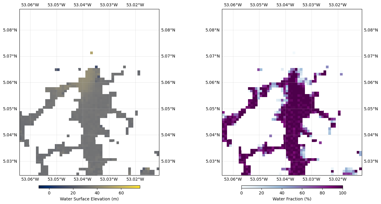
# 1. plot Water Surface Elevation on map
# plot data on the map with pcolor function
cb0 = axs[0].pcolor(
    xr_swot_raster100.longitude,
    xr_swot_raster100.latitude,
    xr_swot_raster100.wse,
    transform=crs,
    cmap='cividis',
    )
# customize plot with pre-defined function
customize_map(axs[0], cb0, "Water Surface Elevation (m)")

# 2. plot Water Fraction on map
cb1 = axs[1].pcolor(
    xr_swot_raster100.longitude,
    xr_swot_raster100.latitude,
    xr_swot_raster100.water_frac*100,
    transform=crs,
    cmap='BuPu',
    vmin=0,
    vmax=100,
    )
# customize plot with pre-defined function
customize_map(axs[1], cb1, "Water Fraction (%)")

/tmp/ipykernel_160234/2149712467.py:21: MatplotlibDeprecationWarning: Getting the array from a PolyQuadMesh will return the full array in the future (uncompressed). To get this behavior now set the PolyQuadMesh with a 2D array .set_array(data2d).
  plt.colorbar(
/tmp/ipykernel_160234/2149712467.py:21: MatplotlibDeprecationWarning: Getting the array from a PolyQuadMesh will return the full array in the future (uncompressed). To get this behavior now set the PolyQuadMesh with a 2D array .set_array(data2d).
  plt.colorbar(

<GeoAxes: >

Download notebook.