Download notebook.

Copyright CNES

Plot a lake timeseries from multiple Lake/River Single Pass products

In this notebook, we show how to read the SWOT-HR River or Lake Single Pass vector products with geopandas and dask dataframes and how to represent a variable in time. The example is based on Lake Single Pass Prior products, but it would be the same methodology for all vector products relying on a feature ID

Libraries

import glob

import numpy as np
import geopandas as gpd
from tqdm import tqdm

from dask import dataframe as dd
from dask.distributed import Client

from datetime import datetime as dt

Select all Lake Single-Pass products within our directory

Filter by filename pattern

filename_list = glob.glob("../docs/data/swot/SWOT_L2_HR_LakeSP_Prior/*PIC0_01/*PIC0_01.zip")
print(len(filename_list))
# one can use zip files, but note it is slower

49

Load all data

now we want to load all data from all file in lazy mode, otherwise it will not fit into RAM.

For this, we will iteratively read all files with geopandas, and store data in a dask dataframe.

With this method, you drop the geometries. If you are fine with that, it is very efficient, otherwise, you can use dask-geopandas instead, see other notebook in the same section.

def get_df(f):
    gdf = gpd.read_file(
        f,
        engine='pyogrio',
        use_arrow=True,
    )
    # RIP geometry or don't drop and use dask_geopandas.from_geopandas instead of dd.from_pandas
    gdf = gdf.drop(columns=['geometry'])
    return gdf


def load_layers(files):
    client = Client()
    futures = client.map(get_df, files)

    ddf = dd.from_delayed(futures)

    return ddf

ddf = load_layers(filename_list)
ddf

Dask DataFrame Structure:

	lake_id	reach_id	obs_id	overlap	n_overlap	time	time_tai	time_str	wse	wse_u	wse_r_u	wse_std	area_total	area_tot_u	area_detct	area_det_u	layovr_val	xtrk_dist	ds1_l	ds1_l_u	ds1_q	ds1_q_u	ds2_l	ds2_l_u	ds2_q	ds2_q_u	quality_f	dark_frac	ice_clim_f	ice_dyn_f	partial_f	xovr_cal_q	geoid_hght	solid_tide	load_tidef	load_tideg	pole_tide	dry_trop_c	wet_trop_c	iono_c	xovr_cal_c	lake_name	p_res_id	p_lon	p_lat	p_ref_wse	p_ref_area	p_date_t0	p_ds_t0	p_storage
npartitions=49
	object	object	object	object	object	float64	float64	object	float64	float64	float64	float64	float64	float64	float64	float64	float64	float64	float64	float64	float64	float64	float64	float64	float64	float64	int32	float64	int32	int32	int32	int32	float64	float64	float64	float64	float64	float64	float64	float64	float64	object	int32	float64	float64	float64	float64	object	float64	float64
	...	...	...	...	...	...	...	...	...	...	...	...	...	...	...	...	...	...	...	...	...	...	...	...	...	...	...	...	...	...	...	...	...	...	...	...	...	...	...	...	...	...	...	...	...	...	...	...	...	...
...	...	...	...	...	...	...	...	...	...	...	...	...	...	...	...	...	...	...	...	...	...	...	...	...	...	...	...	...	...	...	...	...	...	...	...	...	...	...	...	...	...	...	...	...	...	...	...	...	...	...
	...	...	...	...	...	...	...	...	...	...	...	...	...	...	...	...	...	...	...	...	...	...	...	...	...	...	...	...	...	...	...	...	...	...	...	...	...	...	...	...	...	...	...	...	...	...	...	...	...	...
	...	...	...	...	...	...	...	...	...	...	...	...	...	...	...	...	...	...	...	...	...	...	...	...	...	...	...	...	...	...	...	...	...	...	...	...	...	...	...	...	...	...	...	...	...	...	...	...	...	...

Dask Name: fromdelayed, 50 expressions

Focus on our lake of interest

If you do not know the ID of your lake of interest, you can get it the SWOT Prior Lake Database. This database can be viewed and/or downloaded from the hydroweb.next platform. You will find the SWOT Prior Lake Database (PLD) among the ‘Results’ from hydroweb.next. If you do not want to download it, click on “+Project” icon to add it to your project and click on the “EYE” icon to display this vector layer into the current map selection. Note that you may have to place this product on top of the products in your “Project” panel or unselect the “EYE” icon of the other products, in order to view the PLD layer on the map. On the map click inside the water body of interest (here the “river-lake” we are studying) and you will see more details about it in the ‘Select’ panel.

MY_LAKE_ID = '2940020983'

df_vs = ddf[ddf['lake_id'] == MY_LAKE_ID].compute()

# Interpreting the dates as dates with the datetime library
df_vs['time_str'] = df_vs['time_str'].apply(
    lambda t: np.nan if t =='no_data' else dt.fromisoformat(t.strip('Z'))
    )

# sorting values based on dated
df_vs.sort_values('time_str', inplace=True)

# interpreting NaNs (shapefiles have no system to identify fillvalues)
df_vs = df_vs[df_vs['wse']>-1e10]

df_vs

	lake_id	reach_id	obs_id	overlap	n_overlap	time	time_tai	time_str	wse	wse_u	...	xovr_cal_c	lake_name	p_res_id	p_lon	p_lat	p_ref_wse	p_ref_area	p_date_t0	p_ds_t0	p_storage
27845	2940020983	29469100171;29469100181;29469100161;2946910014...	294090L000211;294090L000584;294090L000586;2940...	6;1;1;0;0;0;0;0;0	9	7.618071e+08	7.618072e+08	2024-02-21 05:05:43	308.797	0.060	...	6.006220e-01	no_data	-99999999	42.774543	36.726391	-1.000000e+12	221.719	no_data	-1.000000e+12	-1.000000e+12
29549	2940020983	29469100171;29469100181;29469100161;2946910014...	294090R000212;294090R000175;294090R000187;2940...	2;1;1;1;0;0;0;0;0	9	7.626653e+08	7.626653e+08	2024-03-02 03:27:58	308.357	0.006	...	-2.362345e+00	no_data	-99999999	42.774543	36.726391	-1.000000e+12	221.719	no_data	-1.000000e+12	-1.000000e+12
22681	2940020983	29469100171;29469100181;29469100161;2946910014...	294219R000180;294219R000160;294219R000194;2942...	26;14;3;1;1;0;0;0;0;0	10	7.627129e+08	7.627129e+08	2024-03-02 16:41:13	308.991	0.026	...	-9.724420e-01	no_data	-99999999	42.774543	36.726391	-1.000000e+12	221.719	no_data	-1.000000e+12	-1.000000e+12
29593	2940020983	29469100171;29469100181;29469100161;2946910014...	294090R000695;294090R000580;294090R000609;2940...	2;1;1;1;0;0;0;0;0;0;0	11	7.644680e+08	7.644680e+08	2024-03-23 00:13:01	311.566	0.006	...	-8.630990e-01	no_data	-99999999	42.774543	36.726391	-1.000000e+12	221.719	no_data	-1.000000e+12	-1.000000e+12
27870	2940020983	29469100171;29469100181;29469100161;2946910014...	294090L000101;294090L000069;294090L000100;2940...	4;2;2;2;1;1;1;0;0;0;0;0;0;0;0;0;0;0;0;0;0;0;0;...	26	7.654126e+08	7.654126e+08	2024-04-02 22:35:50	315.545	0.004	...	-1.000000e+12	no_data	-99999999	42.774543	36.726391	-1.000000e+12	221.719	no_data	-1.000000e+12	-1.000000e+12
27873	2940020983	29469100171;29469100181;29469100161;2946910014...	294090L000068;294090L000127;294090L000258;2940...	5;1;1;1;0;0;0;0;0;0;0;0;0;0;0;0;0;0;0;0;0;0;0;...	27	7.672153e+08	7.672153e+08	2024-04-23 19:20:56	320.930	0.007	...	6.728950e-01	no_data	-99999999	42.774543	36.726391	-1.000000e+12	221.719	no_data	-1.000000e+12	-1.000000e+12
29570	2940020983	29469100171;29469100181;29469100161;2946910014...	294090R000446;294090R000379;294090R000393;2940...	2;1;1;1;0;0;0;0;0;0;0	11	7.680734e+08	7.680734e+08	2024-05-03 17:43:09	323.098	0.003	...	6.785700e-02	no_data	-99999999	42.774543	36.726391	-1.000000e+12	221.719	no_data	-1.000000e+12	-1.000000e+12
22680	2940020983	29469100171;29469100181;29469100161;2946910014...	294219R000608;294219R000694;294219R000682;2942...	2;1;1;1;1;0;0;0;0;0;0;0;0;0;0;0	16	7.681210e+08	7.681210e+08	2024-05-04 06:56:25	323.391	0.006	...	4.569000e-03	no_data	-99999999	42.774543	36.726391	-1.000000e+12	221.719	no_data	-1.000000e+12	-1.000000e+12
29544	2940020983	29469100171;29469100181;29469100161;2946910014...	294090R000222;294090R000171;294090R000182;2940...	2;1;1;1;0;0;0;0;0;0;0;0;0	13	7.698761e+08	7.698761e+08	2024-05-24 14:28:15	325.121	0.003	...	7.896590e-01	no_data	-99999999	42.774543	36.726391	-1.000000e+12	221.719	no_data	-1.000000e+12	-1.000000e+12

9 rows × 50 columns

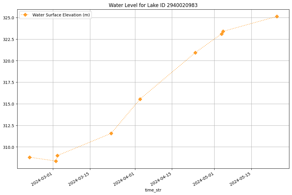
ax = df_vs.plot(
    'time_str',
    'wse',
    label='Water Surface Elevation (m)',
    color='darkorange',
    alpha=.8,
    marker='D',
    ls=':',
    figsize=(12,8),
)
ax.grid(True)
ax.set_title(f'Water Level for Lake ID {MY_LAKE_ID}')

Text(0.5, 1.0, 'Water Level for Lake ID 2940020983')

Download notebook.