Download notebook.

Copyright CNES

Read and plot a SWOT-HR Pixel Cloud netcdf products

In this notebook, we show how to read the SWOT-HR pixel cloud products with xarray and how to represent a variable on a map with cartopy.

Libraries

Please note that apart from the libraries listed in the cell below, you need to install the h5netcdf library (conda install -c conda-forge h5netcdf). This will be used by th xarray.open_dataset function to read the netcdf files.

import xarray as xr
import os
import numpy as np
import matplotlib.pyplot as plt
%matplotlib inline

1. Read a SWOT-HR Pixel Cloud netcdf product

Note this is an extraction of the original file for demonstration purpose. It does not contain all variables and groups

dir_swot = "../docs/data/swot"
file_swot_pxc = os.path.join(dir_swot, "SWOT_L2_HR_PIXC", "SWOT_L2_HR_PIXC_015_033_163R_20240509T115817_20240509T115828_PIC0_01_extract.nc")
# read data with xarray, specifying a group in the netcdf structure
xr_pxc = xr.open_dataset(file_swot_pxc, group="pixel_cloud")

# remove undefined values based on variable of interest
xr_pxc = xr_pxc.where(
    (xr_pxc['classification']>=3) &
    (xr_pxc['sig0']>=20) &
    (xr_pxc['cross_track']>=10000) &
    ~np.isnan(xr_pxc['height'])
)
xr_pxc['wse'] = xr_pxc['height'] - xr_pxc['geoid']
xr_pxc

<xarray.Dataset>
Dimensions:         (points: 10001)
Coordinates:
    latitude        (points) float64 4.597 4.597 4.597 ... 4.653 4.652 4.652
    longitude       (points) float64 -53.06 -53.06 -53.06 ... -53.39 -53.39
Dimensions without coordinates: points
Data variables:
    classification  (points) float32 nan nan nan nan nan ... nan nan nan nan nan
    coherent_power  (points) float32 nan nan nan nan nan ... nan nan nan nan nan
    cross_track     (points) float32 nan nan nan nan nan ... nan nan nan nan nan
    geoid           (points) float32 nan nan nan nan nan ... nan nan nan nan nan
    height          (points) float32 nan nan nan nan nan ... nan nan nan nan nan
    sig0            (points) float32 nan nan nan nan nan ... nan nan nan nan nan
    wse             (points) float32 nan nan nan nan nan ... nan nan nan nan nan
Attributes:
    description:                 cloud of geolocated interferogram pixels
    interferogram_size_azimuth:  3277
    interferogram_size_range:    4694
    looks_to_efflooks:           1.55135648150391
    num_azimuth_looks:           7.0
    azimuth_offset:              7

xarray.Dataset

• Dimensions:
  • points: 10001
• Coordinates: (2)
  • latitude
    (points)
    float64
    4.597 4.597 4.597 ... 4.652 4.652

    long_name :

    latitude (positive N, negative S)

    standard_name :

    latitude

    units :

    degrees_north

    quality_flag :

    geolocation_qual

    valid_min :

    -80.0

    valid_max :

    80.0

    comment :

    Geodetic latitude [-80,80] (degrees north of equator) of the pixel.

    array([4.59743027, 4.5974349 , 4.59737578, ..., 4.65347469, 4.65246108,
           4.6522176 ])

  • longitude
    (points)
    float64
    -53.06 -53.06 ... -53.39 -53.39

    long_name :

    longitude (degrees East)

    standard_name :

    longitude

    units :

    degrees_east

    quality_flag :

    geolocation_qual

    valid_min :

    -180.0

    valid_max :

    180.0

    comment :

    Longitude [-180,180) (east of the Greenwich meridian) of the pixel.

    array([-53.06354572, -53.06357698, -53.06317784, ..., -53.39698461,
           -53.39011959, -53.38847065])

• Data variables: (7)
  • classification
    (points)
    float32
    nan nan nan nan ... nan nan nan nan

    long_name :

    classification

    quality_flag :

    classification_qual

    flag_meanings :

    land land_near_water water_near_land open_water dark_water low_coh_water_near_land open_low_coh_water

    flag_values :

    [1 2 3 4 5 6 7]

    valid_min :

    1

    valid_max :

    7

    comment :

    Flags indicating water detection results.

    array([nan, nan, nan, ..., nan, nan, nan], dtype=float32)

  • coherent_power
    (points)
    float32
    nan nan nan nan ... nan nan nan nan

    long_name :

    coherent power combination of minus_y and plus_y channels

    units :

    1

    quality_flag :

    interferogram_qual

    valid_min :

    0.0

    valid_max :

    1e+20

    comment :

    Power computed by combining the plus_y and minus_y channels coherently by co-aligning the phases (arbitrary units that give sigma0 when noise subtracted and normalized by the X factor).

    array([nan, nan, nan, ..., nan, nan, nan], dtype=float32)

  • cross_track
    (points)
    float32
    nan nan nan nan ... nan nan nan nan

    long_name :

    approximate cross-track location

    units :

    m

    quality_flag :

    geolocation_qual

    valid_min :

    -75000.0

    valid_max :

    75000.0

    comment :

    Approximate cross-track location of the pixel.

    array([nan, nan, nan, ..., nan, nan, nan], dtype=float32)

  • geoid
    (points)
    float32
    nan nan nan nan ... nan nan nan nan

    long_name :

    geoid height

    standard_name :

    geoid_height_above_reference_ellipsoid

    source :

    EGM2008 (Pavlis et al., 2012)

    units :

    m

    valid_min :

    -150.0

    valid_max :

    150.0

    comment :

    Geoid height above the reference ellipsoid with a correction to refer the value to the mean tide system, i.e. includes the permanent tide (zero frequency). This value is reported for reference but is not applied to the reported height.

    array([nan, nan, nan, ..., nan, nan, nan], dtype=float32)

  • height
    (points)
    float32
    nan nan nan nan ... nan nan nan nan

    long_name :

    height above reference ellipsoid

    units :

    m

    quality_flag :

    geolocation_qual

    valid_min :

    -1500.0

    valid_max :

    15000.0

    comment :

    Height of the pixel above the reference ellipsoid.

    array([nan, nan, nan, ..., nan, nan, nan], dtype=float32)

  • sig0
    (points)
    float32
    nan nan nan nan ... nan nan nan nan

    long_name :

    sigma0

    units :

    1

    quality_flag :

    sig0_qual

    valid_min :

    -999999.0

    valid_max :

    999999.0

    comment :

    Normalized radar cross section (sigma0) in real, linear units (not decibels). The value may be negative due to noise subtraction.

    array([nan, nan, nan, ..., nan, nan, nan], dtype=float32)

  • wse
    (points)
    float32
    nan nan nan nan ... nan nan nan nan

    array([nan, nan, nan, ..., nan, nan, nan], dtype=float32)

• Indexes: (0)
• Attributes: (6)

  description :

  cloud of geolocated interferogram pixels

  interferogram_size_azimuth :

  3277

  interferogram_size_range :

  4694

  looks_to_efflooks :

  1.55135648150391

  num_azimuth_looks :

  7.0

  azimuth_offset :

  7

3. Plot data on maps with cartopy

import cartopy.crs as ccrs
import cartopy.feature as cfeature


def customize_map(ax, cb, label, crs=ccrs.PlateCarree()):
    """This function customizes a map with projection and returns the plt.axes instance"""

    ax.gridlines(
        crs=crs,
        draw_labels=True,
        color='.7',
        alpha=.6,
        linewidth=.4,
        linestyle='-',
        )

    # add a background_map (default, local image, WMTS...read the doc)
    # ax.stock_img()

    # add a labeled colorbar
    plt.colorbar(
        cb,
        ax=ax,
        orientation='horizontal',
        shrink=0.6,
        pad=.05,
        aspect=40,
        label=label)

    return ax


# 0. Create Figure and Axes
crs = ccrs.PlateCarree()
fig, ax = plt.subplots(
    subplot_kw={'projection': crs},
    figsize=(12,8),
    frameon=True,
    )

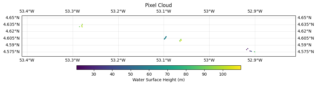
# 1. plot data on the map with scatter function
cb0 = ax.scatter(
    x=xr_pxc.longitude,
    y=xr_pxc.latitude,
    c=xr_pxc.wse,
    s=1,
    transform=crs,
    cmap='viridis',
    )
# Initiate a map with the function above for Pixel cloud
customize_map(ax, cb0, "Water Surface Height (m)")
# limit map boundaries based on actual data
ax.set_extent(
    [
        xr_pxc.longitude.min(),
        xr_pxc.longitude.max(),
        xr_pxc.latitude.min(),
        xr_pxc.latitude.max(),
    ],
    crs=crs
    )
ax.set_title("Pixel Cloud")

Text(0.5, 1.0, 'Pixel Cloud')

Download notebook.