Download notebook.

From the PO.DAAC Cookbook, to access the GitHub version of the notebook, follow this link.

SWOT Hydrology Dataset Exploration on a local machine

Accessing and Visualizing SWOT Datasets

Requirement:

Local compute environment e.g. laptop, server: this tutorial can be run on your local machine.

Learning Objectives:

• Access SWOT HR data prodcuts (archived in NASA Earthdata Cloud) within the AWS cloud, by downloading to local machine

• Visualize accessed data for a quick check

SWOT Level 2 KaRIn High Rate Version 2.0 Datasets:

1. River Vector Shapefile - SWOT_L2_HR_RIVERSP_2.0

2. Lake Vector Shapefile - SWOT_L2_HR_LAKESP_2.0

3. Water Mask Pixel Cloud NetCDF - SWOT_L2_HR_PIXC_2.0

4. Water Mask Pixel Cloud Vector Attribute NetCDF - SWOT_L2_HR_PIXCVec_2.0

5. Raster NetCDF - SWOT_L2_HR_Raster_2.0

6. Single Look Complex Data product - SWOT_L1B_HR_SLC_2.0

Notebook Author: Cassie Nickles, NASA PO.DAAC (Feb 2024) || Other Contributors: Zoe Walschots (PO.DAAC Summer Intern 2023), Catalina Taglialatela (NASA PO.DAAC), Luis Lopez (NASA NSIDC DAAC)

Last updated: 7 Feb 2024

Libraries Needed

import glob
import h5netcdf
import xarray as xr
import pandas as pd
import geopandas as gpd
import contextily as cx
import numpy as np
import matplotlib.pyplot as plt
import hvplot.xarray
import zipfile
import earthaccess

Earthdata Login

An Earthdata Login account is required to access data, as well as discover restricted data, from the NASA Earthdata system. Thus, to access NASA data, you need Earthdata Login. If you don’t already have one, please visit https://urs.earthdata.nasa.gov to register and manage your Earthdata Login account. This account is free to create and only takes a moment to set up. We use earthaccess to authenticate your login credentials below.

auth = earthaccess.login()

Single File Access

1. River Vector Shapefiles

The https access link can be found using earthaccess data search. Since this collection consists of Reach and Node files, we need to extract only the granule for the Reach file. We do this by filtering for the ‘Reach’ title in the data link.

Alternatively, Earthdata Search (see tutorial) can be used to manually search in a GUI interface.

For additional tips on spatial searching of SWOT HR L2 data, see also PO.DAAC Cookbook - SWOT Chapter tips section.

Search for the data of interest

#Retrieves granule from the day we want, in this case by passing to `earthdata.search_data` function the data collection shortname, temporal bounds, and filter by wildcards
river_results = earthaccess.search_data(short_name = 'SWOT_L2_HR_RIVERSP_2.0',
                                        #temporal = ('2024-02-01 00:00:00', '2024-02-29 23:59:59'), # can also specify by time
                                        granule_name = '*Reach*_009_NA*') # here we filter by Reach files (not node), pass=009, continent code=NA

Granules found: 5

Dowload, unzip, read the data

Let’s download the first data file! earthaccess.download has a list as the input format, so we need to put brackets around the single file we pass.

earthaccess.download([river_results[0]], "./data_downloads")

 Getting 1 granules, approx download size: 0.01 GB

['SWOT_L2_HR_RiverSP_Reach_007_009_NA_20231123T172635_20231123T172636_PIC0_01.zip']

The native format for this data is a .zip file, and we want the .shp file within the .zip file, so we must first extract the data to open it. First, we’ll programmatically get the filename we just downloaded, and then extract all data to the data_downloads folder.

filename = earthaccess.results.DataGranule.data_links(river_results[0], access='external')
filename = filename[0].split("/")[-1]
filename

'SWOT_L2_HR_RiverSP_Reach_007_009_NA_20231123T172635_20231123T172636_PIC0_01.zip'

with zipfile.ZipFile(f'data_downloads/{filename}', 'r') as zip_ref:
    zip_ref.extractall('data_downloads')

Open the shapefile using geopandas

filename_shp = filename.replace('.zip','.shp')

SWOT_HR_shp1 = gpd.read_file(f'data_downloads/{filename_shp}')

#view the attribute table
SWOT_HR_shp1

	reach_id	time	time_tai	time_str	p_lat	p_lon	river_name	wse	wse_u	wse_r_u	...	p_wid_var	p_n_nodes	p_dist_out	p_length	p_maf	p_dam_id	p_n_ch_max	p_n_ch_mod	p_low_slp	geometry
0	71224500951	-1.000000e+12	-1.000000e+12	no_data	48.517717	-93.692086	Rainy River	-1.000000e+12	-1.000000e+12	-1.000000e+12	...	1480.031	53	244919.492	10586.381484	-1.000000e+12	0	1	1	0	LINESTRING (-93.76076 48.51651, -93.76035 48.5...
1	71224700013	7.540761e+08	7.540762e+08	2023-11-23T17:35:38Z	48.777900	-93.233350	no_data	3.364954e+02	9.003000e-02	2.290000e-03	...	1239358.412	18	3719.676	3514.736672	-1.000000e+12	0	6	1	0	LINESTRING (-93.21387 48.78466, -93.21403 48.7...
2	71224700021	7.540761e+08	7.540762e+08	2023-11-23T17:35:38Z	48.772163	-93.266891	no_data	3.365123e+02	9.199000e-02	1.902000e-02	...	76609.119	8	5305.752	1586.075688	-1.000000e+12	0	6	1	0	LINESTRING (-93.25587 48.77340, -93.25628 48.7...
3	71224700033	7.540761e+08	7.540762e+08	2023-11-23T17:35:38Z	48.733727	-93.116424	no_data	3.365715e+02	9.068000e-02	1.112000e-02	...	297730.945	20	306795.237	3904.961218	-1.000000e+12	0	3	1	0	LINESTRING (-93.09779 48.73888, -93.09820 48.7...
4	71224700041	7.540761e+08	7.540762e+08	2023-11-23T17:35:38Z	48.720271	-93.113458	no_data	3.364742e+02	9.085000e-02	1.238000e-02	...	0.000	6	302890.276	1203.102119	-1.000000e+12	0	1	1	0	LINESTRING (-93.12101 48.72305, -93.12060 48.7...
...	...	...	...	...	...	...	...	...	...	...	...	...	...	...	...	...	...	...	...	...	...
926	77125000241	7.540756e+08	7.540756e+08	2023-11-23T17:26:38Z	17.960957	-100.025397	no_data	3.560650e+02	1.501928e+02	1.501928e+02	...	864.151	70	464330.310	13953.442643	-1.000000e+12	0	2	1	0	LINESTRING (-100.06409 17.97308, -100.06403 17...
927	77125000254	-1.000000e+12	-1.000000e+12	no_data	17.949648	-99.995193	no_data	-1.000000e+12	-1.000000e+12	-1.000000e+12	...	21491.314	2	464735.375	405.065100	-1.000000e+12	10286	1	1	0	LINESTRING (-99.99547 17.95148, -99.99564 17.9...
928	77125000261	7.540756e+08	7.540756e+08	2023-11-23T17:26:47Z	18.362207	-100.696472	no_data	2.316304e+02	9.208000e-02	1.946000e-02	...	3624.715	56	325106.825	11105.124379	-1.000000e+12	0	4	1	0	LINESTRING (-100.68734 18.40208, -100.68723 18...
929	77125000263	-1.000000e+12	-1.000000e+12	no_data	17.956269	-99.961388	no_data	-1.000000e+12	-1.000000e+12	-1.000000e+12	...	43956.311	49	474450.182	9714.807127	-1.000000e+12	0	2	1	0	LINESTRING (-99.99398 17.94824, -99.99369 17.9...
930	77125000273	-1.000000e+12	-1.000000e+12	no_data	17.952683	-99.906755	no_data	-1.000000e+12	-1.000000e+12	-1.000000e+12	...	283915.163	49	484179.822	9729.640027	-1.000000e+12	0	2	1	0	LINESTRING (-99.93256 17.94746, -99.93273 17.9...

931 rows × 127 columns

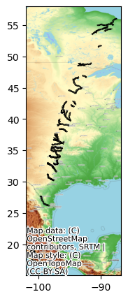
Quickly plot the SWOT river data

# Simple plot
fig, ax = plt.subplots(figsize=(7,5))
SWOT_HR_shp1.plot(ax=ax, color='black')
cx.add_basemap(ax, crs=SWOT_HR_shp1.crs, source=cx.providers.OpenTopoMap)

# Another way to plot geopandas dataframes is with `explore`, which also plots a basemap
#SWOT_HR_shp1.explore()

2. Lake Vector Shapefiles

The lake vector shapefiles can be accessed in the same way as the river shapefiles above.

For additional tips on spatial searching of SWOT HR L2 data, see also PO.DAAC Cookbook - SWOT Chapter tips section.

Search for data of interest

lake_results = earthaccess.search_data(short_name = 'SWOT_L2_HR_LAKESP_2.0',
                                        #temporal = ('2024-02-01 00:00:00', '2024-02-29 23:59:59'), # can also specify by time
                                        granule_name = '*Obs*_009_NA*') # here we filter by files with 'Obs' in the name (This collection has three options: Obs, Unassigned, and Prior), pass #8 and continent code=NA

Granules found: 2

Let’s download the first data file! earthaccess.download has a list as the input format, so we need to put brackets around the single file we pass.

earthaccess.download([lake_results[0]], "./data_downloads")

 Getting 1 granules, approx download size: 0.06 GB

['SWOT_L2_HR_LakeSP_Obs_008_009_NA_20231214T141139_20231214T142322_PIC0_01.zip']

The native format for this data is a .zip file, and we want the .shp file within the .zip file, so we must first extract the data to open it. First, we’ll programmatically get the filename we just downloaded, and then extract all data to the SWOT_downloads folder.

filename2 = earthaccess.results.DataGranule.data_links(lake_results[0], access='external')
filename2 = filename2[0].split("/")[-1]
filename2

'SWOT_L2_HR_LakeSP_Obs_008_009_NA_20231214T141139_20231214T142322_PIC0_01.zip'

with zipfile.ZipFile(f'data_downloads/{filename2}', 'r') as zip_ref:
    zip_ref.extractall('data_downloads')

Open the shapefile using geopandas

filename_shp2 = filename2.replace('.zip','.shp')
filename_shp2

'SWOT_L2_HR_LakeSP_Obs_008_009_NA_20231214T141139_20231214T142322_PIC0_01.shp'

SWOT_HR_shp2 = gpd.read_file(f'data_downloads/{filename_shp2}')

#view the attribute table
SWOT_HR_shp2

	obs_id	lake_id	overlap	n_overlap	reach_id	time	time_tai	time_str	wse	wse_u	...	load_tidef	load_tideg	pole_tide	dry_trop_c	wet_trop_c	iono_c	xovr_cal_c	lake_name	p_res_id	geometry
0	771190L999978	7710050732;7710050703;7710050672;7710050662;77...	9;86;79;70;65	5	no_data	7.558783e+08	7.558783e+08	2023-12-14T14:12:29Z	1888.880	0.002	...	-0.016630	-0.018661	0.004459	-1.865485	-0.153819	-0.005181	-1.116717	PRESA SOLS	-99999999	MULTIPOLYGON (((-100.49406 20.07574, -100.4938...
1	752199L999957	7520013722;7520013783	66;17	2	no_data	7.558784e+08	7.558784e+08	2023-12-14T14:14:08Z	156.216	0.034	...	-0.014181	-0.015942	0.005326	-2.293956	-0.252575	-0.004943	-0.351363	no_data	-99999999	MULTIPOLYGON (((-99.37239 25.63900, -99.37194 ...
2	752200L999987	7520013712	59	1	no_data	7.558784e+08	7.558784e+08	2023-12-14T14:14:09Z	171.336	0.095	...	-0.014314	-0.016066	0.005341	-2.289045	-0.249914	-0.004935	-0.555793	no_data	-99999999	MULTIPOLYGON (((-99.39476 25.73965, -99.39442 ...
3	752200L999975	7520010832	75	1	no_data	7.558784e+08	7.558784e+08	2023-12-14T14:14:09Z	173.704	0.092	...	-0.014527	-0.016270	0.005346	-2.288555	-0.249523	-0.004927	-0.880471	no_data	-99999999	MULTIPOLYGON (((-99.49457 25.75364, -99.49435 ...
4	752201L999995	7520010502	97	1	no_data	7.558785e+08	7.558785e+08	2023-12-14T14:14:20Z	86.140	0.183	...	-0.014221	-0.015947	0.005429	-2.310065	-0.251561	-0.004908	-0.461625	no_data	-99999999	MULTIPOLYGON (((-99.18978 26.22343, -99.18885 ...
...	...	...	...	...	...	...	...	...	...	...	...	...	...	...	...	...	...	...	...	...	...
24067	713255R000242	7131518382	98	1	no_data	7.558790e+08	7.558790e+08	2023-12-14T14:23:21Z	8.600	0.058	...	-0.003146	-0.002480	0.008959	-2.268371	-0.101818	-0.002132	0.371395	no_data	-99999999	POLYGON ((-88.09984 56.45882, -88.09993 56.458...
24068	713255R000243	7131518562	88	1	no_data	7.558790e+08	7.558790e+08	2023-12-14T14:23:21Z	7.569	0.046	...	-0.002484	-0.002016	0.011788	-2.268953	-0.101874	-0.002134	0.536599	no_data	-99999999	POLYGON ((-88.02194 56.44447, -88.02154 56.444...
24069	713255R000252	7131519822	96	1	no_data	7.558790e+08	7.558790e+08	2023-12-14T14:23:21Z	7.010	0.056	...	-0.002542	-0.002187	0.010853	-2.268864	-0.101836	-0.002132	0.410241	no_data	-99999999	POLYGON ((-88.07451 56.46812, -88.07396 56.467...
24070	713255R000253	7131519842	92	1	no_data	7.558790e+08	7.558790e+08	2023-12-14T14:23:21Z	4.540	0.118	...	-0.001758	-0.001693	0.012287	-2.269519	-0.101934	-0.002135	0.580966	no_data	-99999999	POLYGON ((-87.98967 56.45438, -87.98932 56.454...
24071	713255R000256	7131524362	61	1	no_data	7.558790e+08	7.558790e+08	2023-12-14T14:23:21Z	5.420	0.108	...	-0.001757	-0.001759	0.012288	-2.269569	-0.101906	-0.002133	0.503179	no_data	-99999999	POLYGON ((-88.02147 56.47136, -88.02104 56.471...

24072 rows × 36 columns

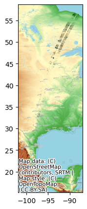
Quickly plot the SWOT lakes data

fig, ax = plt.subplots(figsize=(7,5))
SWOT_HR_shp2.plot(ax=ax, color='black')
cx.add_basemap(ax, crs=SWOT_HR_shp2.crs, source=cx.providers.OpenTopoMap)

Accessing the remaining files is different than the shp files above. We do not need to extract the shapefiles from a zip file because the following SWOT HR collections are stored in netCDF files in the cloud. For the rest of the products, we will open via xarray, not geopandas.

3. Water Mask Pixel Cloud NetCDF

Search for data collection and time of interest

pixc_results = earthaccess.search_data(short_name = 'SWOT_L2_HR_PIXC_2.0',
                                        #granule_name = '*_009_*', # pass number 9 if we want to filter further
                                        #temporal = ('2024-02-01 00:00:00', '2024-02-29 23:59:59'), # can also specify by time
                                        bounding_box = (-106.62, 38.809, -106.54, 38.859)) # Lake Travis near Austin, TX

Granules found: 18

Let’s download one data file! earthaccess.download has a list as the input format, so we need to put brackets around the single file we pass.

earthaccess.download([pixc_results[0]], "./data_downloads")

 Getting 1 granules, approx download size: 0.27 GB

['SWOT_L2_HR_PIXC_007_106_086R_20231127T042024_20231127T042035_PIC0_03.nc']

Open data using xarray

The pixel cloud netCDF files are formatted with three groups titled, “pixel cloud”, “tvp”, or “noise” (more detail here). In order to access the coordinates and variables within the file, a group must be specified when calling xarray open_dataset.

ds_PIXC = xr.open_mfdataset("data_downloads/SWOT_L2_HR_PIXC_*.nc", group = 'pixel_cloud', engine='h5netcdf')
ds_PIXC

<xarray.Dataset>
Dimensions:                                (points: 2831150, complex_depth: 2,
                                            num_pixc_lines: 3279)
Coordinates:
    latitude                               (points) float64 dask.array<chunksize=(2831150,), meta=np.ndarray>
    longitude                              (points) float64 dask.array<chunksize=(2831150,), meta=np.ndarray>
Dimensions without coordinates: points, complex_depth, num_pixc_lines
Data variables: (12/61)
    azimuth_index                          (points) float64 dask.array<chunksize=(2831150,), meta=np.ndarray>
    range_index                            (points) float64 dask.array<chunksize=(2831150,), meta=np.ndarray>
    interferogram                          (points, complex_depth) float32 dask.array<chunksize=(2831150, 2), meta=np.ndarray>
    power_plus_y                           (points) float32 dask.array<chunksize=(2831150,), meta=np.ndarray>
    power_minus_y                          (points) float32 dask.array<chunksize=(2831150,), meta=np.ndarray>
    coherent_power                         (points) float32 dask.array<chunksize=(2831150,), meta=np.ndarray>
    ...                                     ...
    pixc_line_qual                         (num_pixc_lines) float64 dask.array<chunksize=(3279,), meta=np.ndarray>
    pixc_line_to_tvp                       (num_pixc_lines) float32 dask.array<chunksize=(3279,), meta=np.ndarray>
    data_window_first_valid                (num_pixc_lines) float64 dask.array<chunksize=(3279,), meta=np.ndarray>
    data_window_last_valid                 (num_pixc_lines) float64 dask.array<chunksize=(3279,), meta=np.ndarray>
    data_window_first_cross_track          (num_pixc_lines) float32 dask.array<chunksize=(3279,), meta=np.ndarray>
    data_window_last_cross_track           (num_pixc_lines) float32 dask.array<chunksize=(3279,), meta=np.ndarray>
Attributes:
    description:                 cloud of geolocated interferogram pixels
    interferogram_size_azimuth:  3279
    interferogram_size_range:    5750
    looks_to_efflooks:           1.5509548020673398
    num_azimuth_looks:           7.0
    azimuth_offset:              3

xarray.Dataset

• Dimensions:
  • points: 2831150
  • complex_depth: 2
  • num_pixc_lines: 3279
• Coordinates: (2)
  • latitude
    (points)
    float64
    dask.array<chunksize=(2831150,), meta=np.ndarray>

    long_name :

    latitude (positive N, negative S)

    standard_name :

    latitude

    units :

    degrees_north

    quality_flag :

    geolocation_qual

    valid_min :

    -80.0

    valid_max :

    80.0

    comment :

    Geodetic latitude [-80,80] (degrees north of equator) of the pixel.

    Array Chunk Bytes 22.65 MB 22.65 MB Shape (2831150,) (2831150,) Count 2 Tasks 1 Chunks Type float64 numpy.ndarray

  • longitude
    (points)
    float64
    dask.array<chunksize=(2831150,), meta=np.ndarray>

    long_name :

    longitude (degrees East)

    standard_name :

    longitude

    units :

    degrees_east

    quality_flag :

    geolocation_qual

    valid_min :

    -180.0

    valid_max :

    180.0

    comment :

    Longitude [-180,180) (east of the Greenwich meridian) of the pixel.

    Array Chunk Bytes 22.65 MB 22.65 MB Shape (2831150,) (2831150,) Count 2 Tasks 1 Chunks Type float64 numpy.ndarray

• Data variables: (61)
  • azimuth_index
    (points)
    float64
    dask.array<chunksize=(2831150,), meta=np.ndarray>

    long_name :

    rare interferogram azimuth index

    units :

    1

    valid_min :

    0

    valid_max :

    999999

    comment :

    Rare interferogram azimuth index (indexed from 0).

    Array Chunk Bytes 22.65 MB 22.65 MB Shape (2831150,) (2831150,) Count 2 Tasks 1 Chunks Type float64 numpy.ndarray

  • range_index
    (points)
    float64
    dask.array<chunksize=(2831150,), meta=np.ndarray>

    long_name :

    rare interferogram range index

    units :

    1

    valid_min :

    0

    valid_max :

    999999

    comment :

    Rare interferogram range index (indexed from 0).

    Array Chunk Bytes 22.65 MB 22.65 MB Shape (2831150,) (2831150,) Count 2 Tasks 1 Chunks Type float64 numpy.ndarray

  • interferogram
    (points, complex_depth)
    float32
    dask.array<chunksize=(2831150, 2), meta=np.ndarray>

    long_name :

    rare interferogram

    units :

    1

    quality_flag :

    interferogram_qual

    valid_min :

    -1e+20

    valid_max :

    1e+20

    comment :

    Complex unflattened rare interferogram.

    Array Chunk Bytes 22.65 MB 22.65 MB Shape (2831150, 2) (2831150, 2) Count 2 Tasks 1 Chunks Type float32 numpy.ndarray

  • power_plus_y
    (points)
    float32
    dask.array<chunksize=(2831150,), meta=np.ndarray>

    long_name :

    power for plus_y channel

    units :

    1

    quality_flag :

    interferogram_qual

    valid_min :

    0.0

    valid_max :

    1e+20

    comment :

    Power for the plus_y channel (arbitrary units that give sigma0 when noise subtracted and normalized by the X factor).

    Array Chunk Bytes 11.32 MB 11.32 MB Shape (2831150,) (2831150,) Count 2 Tasks 1 Chunks Type float32 numpy.ndarray

  • power_minus_y
    (points)
    float32
    dask.array<chunksize=(2831150,), meta=np.ndarray>

    long_name :

    power for minus_y channel

    units :

    1

    quality_flag :

    interferogram_qual

    valid_min :

    0.0

    valid_max :

    1e+20

    comment :

    Power for the minus_y channel (arbitrary units that give sigma0 when noise subtracted and normalized by the X factor).

    Array Chunk Bytes 11.32 MB 11.32 MB Shape (2831150,) (2831150,) Count 2 Tasks 1 Chunks Type float32 numpy.ndarray

  • coherent_power
    (points)
    float32
    dask.array<chunksize=(2831150,), meta=np.ndarray>

    long_name :

    coherent power combination of minus_y and plus_y channels

    units :

    1

    quality_flag :

    interferogram_qual

    valid_min :

    0.0

    valid_max :

    1e+20

    comment :

    Power computed by combining the plus_y and minus_y channels coherently by co-aligning the phases (arbitrary units that give sigma0 when noise subtracted and normalized by the X factor).

    Array Chunk Bytes 11.32 MB 11.32 MB Shape (2831150,) (2831150,) Count 2 Tasks 1 Chunks Type float32 numpy.ndarray

  • x_factor_plus_y
    (points)
    float32
    dask.array<chunksize=(2831150,), meta=np.ndarray>

    long_name :

    X factor for plus_y channel power

    units :

    1

    valid_min :

    0.0

    valid_max :

    1e+20

    comment :

    X factor for the plus_y channel power in linear units (arbitrary units to normalize noise-subtracted power to sigma0).

    Array Chunk Bytes 11.32 MB 11.32 MB Shape (2831150,) (2831150,) Count 2 Tasks 1 Chunks Type float32 numpy.ndarray

  • x_factor_minus_y
    (points)
    float32
    dask.array<chunksize=(2831150,), meta=np.ndarray>

    long_name :

    X factor for minus_y channel power

    units :

    1

    valid_min :

    0.0

    valid_max :

    1e+20

    comment :

    X factor for the minus_y channel power in linear units (arbitrary units to normalize noise-subtracted power to sigma0).

    Array Chunk Bytes 11.32 MB 11.32 MB Shape (2831150,) (2831150,) Count 2 Tasks 1 Chunks Type float32 numpy.ndarray

  • water_frac
    (points)
    float32
    dask.array<chunksize=(2831150,), meta=np.ndarray>

    long_name :

    water fraction

    units :

    1

    quality_flag :

    classification_qual

    valid_min :

    -1000.0

    valid_max :

    10000.0

    comment :

    Noisy estimate of the fraction of the pixel that is water.

    Array Chunk Bytes 11.32 MB 11.32 MB Shape (2831150,) (2831150,) Count 2 Tasks 1 Chunks Type float32 numpy.ndarray

  • water_frac_uncert
    (points)
    float32
    dask.array<chunksize=(2831150,), meta=np.ndarray>

    long_name :

    water fraction uncertainty

    units :

    1

    valid_min :

    0.0

    valid_max :

    999999.0

    comment :

    Uncertainty estimate of the water fraction estimate (width of noisy water frac estimate distribution).

    Array Chunk Bytes 11.32 MB 11.32 MB Shape (2831150,) (2831150,) Count 2 Tasks 1 Chunks Type float32 numpy.ndarray

  • classification
    (points)
    float32
    dask.array<chunksize=(2831150,), meta=np.ndarray>

    long_name :

    classification

    quality_flag :

    classification_qual

    flag_meanings :

    land land_near_water water_near_land open_water dark_water low_coh_water_near_land open_low_coh_water

    flag_values :

    [1 2 3 4 5 6 7]

    valid_min :

    1

    valid_max :

    7

    comment :

    Flags indicating water detection results.

    Array Chunk Bytes 11.32 MB 11.32 MB Shape (2831150,) (2831150,) Count 2 Tasks 1 Chunks Type float32 numpy.ndarray

  • false_detection_rate
    (points)
    float32
    dask.array<chunksize=(2831150,), meta=np.ndarray>

    long_name :

    false detection rate

    units :

    1

    quality_flag :

    classification_qual

    valid_min :

    0.0

    valid_max :

    1.0

    comment :

    Probability of falsely detecting water when there is none.

    Array Chunk Bytes 11.32 MB 11.32 MB Shape (2831150,) (2831150,) Count 2 Tasks 1 Chunks Type float32 numpy.ndarray

  • missed_detection_rate
    (points)
    float32
    dask.array<chunksize=(2831150,), meta=np.ndarray>

    long_name :

    missed detection rate

    units :

    1

    quality_flag :

    classification_qual

    valid_min :

    0.0

    valid_max :

    1.0

    comment :

    Probability of falsely detecting no water when there is water.

    Array Chunk Bytes 11.32 MB 11.32 MB Shape (2831150,) (2831150,) Count 2 Tasks 1 Chunks Type float32 numpy.ndarray

  • prior_water_prob
    (points)
    float32
    dask.array<chunksize=(2831150,), meta=np.ndarray>

    long_name :

    prior water probability

    units :

    1

    valid_min :

    0.0

    valid_max :

    1.0

    comment :

    Prior probability of water occurring.

    Array Chunk Bytes 11.32 MB 11.32 MB Shape (2831150,) (2831150,) Count 2 Tasks 1 Chunks Type float32 numpy.ndarray

  • bright_land_flag
    (points)
    float32
    dask.array<chunksize=(2831150,), meta=np.ndarray>

    long_name :

    bright land flag

    standard_name :

    status_flag

    flag_meanings :

    not_bright_land bright_land bright_land_or_water

    flag_values :

    [0 1 2]

    valid_min :

    0

    valid_max :

    2

    comment :

    Flag indicating areas that are not typically water but are expected to be bright (e.g., urban areas, ice). Flag value 2 indicates cases where prior data indicate land, but where prior_water_prob indicates possible water.

    Array Chunk Bytes 11.32 MB 11.32 MB Shape (2831150,) (2831150,) Count 2 Tasks 1 Chunks Type float32 numpy.ndarray

  • layover_impact
    (points)
    float32
    dask.array<chunksize=(2831150,), meta=np.ndarray>

    long_name :

    layover impact

    units :

    m

    valid_min :

    -999999.0

    valid_max :

    999999.0

    comment :

    Estimate of the height error caused by layover, which may not be reliable on a pixel by pixel basis, but may be useful to augment aggregated height uncertainties.

    Array Chunk Bytes 11.32 MB 11.32 MB Shape (2831150,) (2831150,) Count 2 Tasks 1 Chunks Type float32 numpy.ndarray

  • eff_num_rare_looks
    (points)
    float32
    dask.array<chunksize=(2831150,), meta=np.ndarray>

    long_name :

    effective number of rare looks

    units :

    1

    valid_min :

    0.0

    valid_max :

    999999.0

    comment :

    Effective number of independent looks taken to form the rare interferogram.

    Array Chunk Bytes 11.32 MB 11.32 MB Shape (2831150,) (2831150,) Count 2 Tasks 1 Chunks Type float32 numpy.ndarray

  • height
    (points)
    float32
    dask.array<chunksize=(2831150,), meta=np.ndarray>

    long_name :

    height above reference ellipsoid

    units :

    m

    quality_flag :

    geolocation_qual

    valid_min :

    -1500.0

    valid_max :

    15000.0

    comment :

    Height of the pixel above the reference ellipsoid.

    Array Chunk Bytes 11.32 MB 11.32 MB Shape (2831150,) (2831150,) Count 2 Tasks 1 Chunks Type float32 numpy.ndarray

  • cross_track
    (points)
    float32
    dask.array<chunksize=(2831150,), meta=np.ndarray>

    long_name :

    approximate cross-track location

    units :

    m

    quality_flag :

    geolocation_qual

    valid_min :

    -75000.0

    valid_max :

    75000.0

    comment :

    Approximate cross-track location of the pixel.

    Array Chunk Bytes 11.32 MB 11.32 MB Shape (2831150,) (2831150,) Count 2 Tasks 1 Chunks Type float32 numpy.ndarray

  • pixel_area
    (points)
    float32
    dask.array<chunksize=(2831150,), meta=np.ndarray>

    long_name :

    pixel area

    units :

    m^2

    quality_flag :

    geolocation_qual

    valid_min :

    0.0

    valid_max :

    999999.0

    comment :

    Pixel area.

    Array Chunk Bytes 11.32 MB 11.32 MB Shape (2831150,) (2831150,) Count 2 Tasks 1 Chunks Type float32 numpy.ndarray

  • inc
    (points)
    float32
    dask.array<chunksize=(2831150,), meta=np.ndarray>

    long_name :

    incidence angle

    units :

    degrees

    quality_flag :

    geolocation_qual

    valid_min :

    0.0

    valid_max :

    999999.0

    comment :

    Incidence angle.

    Array Chunk Bytes 11.32 MB 11.32 MB Shape (2831150,) (2831150,) Count 2 Tasks 1 Chunks Type float32 numpy.ndarray

  • phase_noise_std
    (points)
    float32
    dask.array<chunksize=(2831150,), meta=np.ndarray>

    long_name :

    phase noise standard deviation

    units :

    radians

    valid_min :

    -999999.0

    valid_max :

    999999.0

    comment :

    Estimate of the phase noise standard deviation.

    Array Chunk Bytes 11.32 MB 11.32 MB Shape (2831150,) (2831150,) Count 2 Tasks 1 Chunks Type float32 numpy.ndarray

  • dlatitude_dphase
    (points)
    float32
    dask.array<chunksize=(2831150,), meta=np.ndarray>

    long_name :

    sensitivity of latitude estimate to interferogram phase

    units :

    degrees/radian

    quality_flag :

    geolocation_qual

    valid_min :

    -999999.0

    valid_max :

    999999.0

    comment :

    Sensitivity of the latitude estimate to the interferogram phase.

    Array Chunk Bytes 11.32 MB 11.32 MB Shape (2831150,) (2831150,) Count 2 Tasks 1 Chunks Type float32 numpy.ndarray

  • dlongitude_dphase
    (points)
    float32
    dask.array<chunksize=(2831150,), meta=np.ndarray>

    long_name :

    sensitivity of longitude estimate to interferogram phase

    units :

    degrees/radian

    quality_flag :

    geolocation_qual

    valid_min :

    -999999.0

    valid_max :

    999999.0

    comment :

    Sensitivity of the longitude estimate to the interferogram phase.

    Array Chunk Bytes 11.32 MB 11.32 MB Shape (2831150,) (2831150,) Count 2 Tasks 1 Chunks Type float32 numpy.ndarray

  • dheight_dphase
    (points)
    float32
    dask.array<chunksize=(2831150,), meta=np.ndarray>

    long_name :

    sensitivity of height estimate to interferogram phase

    units :

    m/radian

    quality_flag :

    geolocation_qual

    valid_min :

    -999999.0

    valid_max :

    999999.0

    comment :

    Sensitivity of the height estimate to the interferogram phase.

    Array Chunk Bytes 11.32 MB 11.32 MB Shape (2831150,) (2831150,) Count 2 Tasks 1 Chunks Type float32 numpy.ndarray

  • dheight_droll
    (points)
    float32
    dask.array<chunksize=(2831150,), meta=np.ndarray>

    long_name :

    sensitivity of height estimate to spacecraft roll

    units :

    m/degrees

    quality_flag :

    geolocation_qual

    valid_min :

    -999999.0

    valid_max :

    999999.0

    comment :

    Sensitivity of the height estimate to the spacecraft roll.

    Array Chunk Bytes 11.32 MB 11.32 MB Shape (2831150,) (2831150,) Count 2 Tasks 1 Chunks Type float32 numpy.ndarray

  • dheight_dbaseline
    (points)
    float32
    dask.array<chunksize=(2831150,), meta=np.ndarray>

    long_name :

    sensitivity of height estimate to interferometric baseline

    units :

    m/m

    quality_flag :

    geolocation_qual

    valid_min :

    -999999.0

    valid_max :

    999999.0

    comment :

    Sensitivity of the height estimate to the interferometric baseline.

    Array Chunk Bytes 11.32 MB 11.32 MB Shape (2831150,) (2831150,) Count 2 Tasks 1 Chunks Type float32 numpy.ndarray

  • dheight_drange
    (points)
    float32
    dask.array<chunksize=(2831150,), meta=np.ndarray>

    long_name :

    sensitivity of height estimate to range (delay)

    units :

    m/m

    quality_flag :

    geolocation_qual

    valid_min :

    -999999.0

    valid_max :

    999999.0

    comment :

    Sensitivity of the height estimate to the range (delay).

    Array Chunk Bytes 11.32 MB 11.32 MB Shape (2831150,) (2831150,) Count 2 Tasks 1 Chunks Type float32 numpy.ndarray

  • darea_dheight
    (points)
    float32
    dask.array<chunksize=(2831150,), meta=np.ndarray>

    long_name :

    sensitivity of pixel area to reference height

    units :

    m^2/m

    quality_flag :

    geolocation_qual

    valid_min :

    -999999.0

    valid_max :

    999999.0

    comment :

    Sensitivity of the pixel area to the reference height.

    Array Chunk Bytes 11.32 MB 11.32 MB Shape (2831150,) (2831150,) Count 2 Tasks 1 Chunks Type float32 numpy.ndarray

  • illumination_time
    (points)
    datetime64[ns]
    dask.array<chunksize=(2831150,), meta=np.ndarray>

    long_name :

    time of illumination of each pixel (UTC)

    standard_name :

    time

    tai_utc_difference :

    37.0

    leap_second :

    0000-00-00T00:00:00Z

    comment :

    Time of measurement in seconds in the UTC time scale since 1 Jan 2000 00:00:00 UTC. [tai_utc_difference] is the difference between TAI and UTC reference time (seconds) for the first measurement of the data set. If a leap second occurs within the data set, the attribute leap_second is set to the UTC time at which the leap second occurs.

    Array Chunk Bytes 22.65 MB 22.65 MB Shape (2831150,) (2831150,) Count 2 Tasks 1 Chunks Type datetime64[ns] numpy.ndarray

  • illumination_time_tai
    (points)
    datetime64[ns]
    dask.array<chunksize=(2831150,), meta=np.ndarray>

    long_name :

    time of illumination of each pixel (TAI)

    standard_name :

    time

    comment :

    Time of measurement in seconds in the TAI time scale since 1 Jan 2000 00:00:00 TAI. This time scale contains no leap seconds. The difference (in seconds) with time in UTC is given by the attribute [illumination_time:tai_utc_difference].

    Array Chunk Bytes 22.65 MB 22.65 MB Shape (2831150,) (2831150,) Count 2 Tasks 1 Chunks Type datetime64[ns] numpy.ndarray

  • eff_num_medium_looks
    (points)
    float32
    dask.array<chunksize=(2831150,), meta=np.ndarray>

    long_name :

    effective number of medium looks

    units :

    1

    valid_min :

    0.0

    valid_max :

    999999.0

    comment :

    Effective number of independent looks taken in forming the medium interferogram (after adaptive averaging).

    Array Chunk Bytes 11.32 MB 11.32 MB Shape (2831150,) (2831150,) Count 2 Tasks 1 Chunks Type float32 numpy.ndarray

  • sig0
    (points)
    float32
    dask.array<chunksize=(2831150,), meta=np.ndarray>

    long_name :

    sigma0

    units :

    1

    quality_flag :

    sig0_qual

    valid_min :

    -999999.0

    valid_max :

    999999.0

    comment :

    Normalized radar cross section (sigma0) in real, linear units (not decibels). The value may be negative due to noise subtraction.

    Array Chunk Bytes 11.32 MB 11.32 MB Shape (2831150,) (2831150,) Count 2 Tasks 1 Chunks Type float32 numpy.ndarray

  • sig0_uncert
    (points)
    float32
    dask.array<chunksize=(2831150,), meta=np.ndarray>

    long_name :

    sigma0 uncertainty

    units :

    1

    valid_min :

    -999999.0

    valid_max :

    999999.0

    comment :

    1-sigma uncertainty in the sig0 measurement. The value is given as an additive (not multiplicative) linear term (not a term in decibels).

    Array Chunk Bytes 11.32 MB 11.32 MB Shape (2831150,) (2831150,) Count 2 Tasks 1 Chunks Type float32 numpy.ndarray

  • phase_unwrapping_region
    (points)
    float64
    dask.array<chunksize=(2831150,), meta=np.ndarray>

    long_name :

    phase unwrapping region index

    units :

    1

    valid_min :

    -1

    valid_max :

    99999999

    comment :

    Phase unwrapping region index.

    Array Chunk Bytes 22.65 MB 22.65 MB Shape (2831150,) (2831150,) Count 2 Tasks 1 Chunks Type float64 numpy.ndarray

  • ambiguity_cost1
    (points)
    float32
    dask.array<chunksize=(2831150,), meta=np.ndarray>

    long_name :

    phase ambiguity minimum cost

    units :

    1

    valid_min :

    -999999.0

    valid_max :

    999999.0

    comment :

    Phase ambiguity minimum cost.

    Array Chunk Bytes 11.32 MB 11.32 MB Shape (2831150,) (2831150,) Count 2 Tasks 1 Chunks Type float32 numpy.ndarray

  • ambiguity_cost2
    (points)
    float32
    dask.array<chunksize=(2831150,), meta=np.ndarray>

    long_name :

    phase ambiguity 2nd minimum cost

    units :

    1

    valid_min :

    -999999.0

    valid_max :

    999999.0

    comment :

    Phase ambiguity 2nd minimum cost.

    Array Chunk Bytes 11.32 MB 11.32 MB Shape (2831150,) (2831150,) Count 2 Tasks 1 Chunks Type float32 numpy.ndarray

  • instrument_range_cor
    (points)
    float32
    dask.array<chunksize=(2831150,), meta=np.ndarray>

    long_name :

    instrument range correction

    units :

    m

    valid_min :

    -999999.0

    valid_max :

    999999.0

    comment :

    Term that incorporates all calibration corrections applied to range before geolocation.

    Array Chunk Bytes 11.32 MB 11.32 MB Shape (2831150,) (2831150,) Count 2 Tasks 1 Chunks Type float32 numpy.ndarray

  • instrument_phase_cor
    (points)
    float32
    dask.array<chunksize=(2831150,), meta=np.ndarray>

    long_name :

    instrument phase correction

    units :

    radians

    valid_min :

    -999999.0

    valid_max :

    999999.0

    comment :

    Term that incorporates all calibration corrections applied to phase before geolocation.

    Array Chunk Bytes 11.32 MB 11.32 MB Shape (2831150,) (2831150,) Count 2 Tasks 1 Chunks Type float32 numpy.ndarray

  • instrument_baseline_cor
    (points)
    float32
    dask.array<chunksize=(2831150,), meta=np.ndarray>

    long_name :

    instrument baseline correction

    units :

    m

    valid_min :

    -999999.0

    valid_max :

    999999.0

    comment :

    Term that incorporates all calibration corrections applied to baseline before geolocation.

    Array Chunk Bytes 11.32 MB 11.32 MB Shape (2831150,) (2831150,) Count 2 Tasks 1 Chunks Type float32 numpy.ndarray

  • sig0_cor_atmos_model
    (points)
    float32
    dask.array<chunksize=(2831150,), meta=np.ndarray>

    long_name :

    two-way atmospheric correction to sigma0 from model

    source :

    European Centre for Medium-Range Weather Forecasts

    institution :

    ECMWF

    units :

    1

    valid_min :

    1.0

    valid_max :

    10.0

    comment :

    Atmospheric correction to sigma0 from weather model data as a linear power multiplier (not decibels). sig0_cor_atmos_model is already applied in computing sig0 and x_factor_plus_y and x_factor_minus_y.

    Array Chunk Bytes 11.32 MB 11.32 MB Shape (2831150,) (2831150,) Count 2 Tasks 1 Chunks Type float32 numpy.ndarray

  • height_cor_xover
    (points)
    float32
    dask.array<chunksize=(2831150,), meta=np.ndarray>

    long_name :

    height correction from KaRIn crossovers

    units :

    m

    valid_min :

    -10.0

    valid_max :

    10.0

    comment :

    Height correction from KaRIn crossover calibration. The correction is applied before geolocation but reported as an equivalent height correction.

    Array Chunk Bytes 11.32 MB 11.32 MB Shape (2831150,) (2831150,) Count 2 Tasks 1 Chunks Type float32 numpy.ndarray

  • model_dry_tropo_cor
    (points)
    float32
    dask.array<chunksize=(2831150,), meta=np.ndarray>

    long_name :

    dry troposphere vertical correction

    source :

    European Centre for Medium-Range Weather Forecasts

    institution :

    ECMWF

    units :

    m

    valid_min :

    -3.0

    valid_max :

    -1.5

    comment :

    Equivalent vertical correction due to dry troposphere delay. The reported pixel height, latitude and longitude are computed after adding negative media corrections to uncorrected range along slant-range paths, accounting for the differential delay between the two KaRIn antennas. The equivalent vertical correction is computed by applying obliquity factors to the slant-path correction. Adding the reported correction to the reported pixel height results in the uncorrected pixel height.

    Array Chunk Bytes 11.32 MB 11.32 MB Shape (2831150,) (2831150,) Count 2 Tasks 1 Chunks Type float32 numpy.ndarray

  • model_wet_tropo_cor
    (points)
    float32
    dask.array<chunksize=(2831150,), meta=np.ndarray>

    long_name :

    wet troposphere vertical correction

    source :

    European Centre for Medium-Range Weather Forecasts

    institution :

    ECMWF

    units :

    m

    valid_min :

    -1.0

    valid_max :

    0.0

    comment :

    Equivalent vertical correction due to wet troposphere delay. The reported pixel height, latitude and longitude are computed after adding negative media corrections to uncorrected range along slant-range paths, accounting for the differential delay between the two KaRIn antennas. The equivalent vertical correction is computed by applying obliquity factors to the slant-path correction. Adding the reported correction to the reported pixel height results in the uncorrected pixel height.

    Array Chunk Bytes 11.32 MB 11.32 MB Shape (2831150,) (2831150,) Count 2 Tasks 1 Chunks Type float32 numpy.ndarray

  • iono_cor_gim_ka
    (points)
    float32
    dask.array<chunksize=(2831150,), meta=np.ndarray>

    long_name :

    ionosphere vertical correction

    source :

    Global Ionosphere Maps

    institution :

    JPL

    units :

    m

    valid_min :

    -0.5

    valid_max :

    0.0

    comment :

    Equivalent vertical correction due to ionosphere delay. The reported pixel height, latitude and longitude are computed after adding negative media corrections to uncorrected range along slant-range paths, accounting for the differential delay between the two KaRIn antennas. The equivalent vertical correction is computed by applying obliquity factors to the slant-path correction. Adding the reported correction to the reported pixel height results in the uncorrected pixel height.

    Array Chunk Bytes 11.32 MB 11.32 MB Shape (2831150,) (2831150,) Count 2 Tasks 1 Chunks Type float32 numpy.ndarray

  • geoid
    (points)
    float32
    dask.array<chunksize=(2831150,), meta=np.ndarray>

    long_name :

    geoid height

    standard_name :

    geoid_height_above_reference_ellipsoid

    source :

    EGM2008 (Pavlis et al., 2012)

    units :

    m

    valid_min :

    -150.0

    valid_max :

    150.0

    comment :

    Geoid height above the reference ellipsoid with a correction to refer the value to the mean tide system, i.e. includes the permanent tide (zero frequency). This value is reported for reference but is not applied to the reported height.

    Array Chunk Bytes 11.32 MB 11.32 MB Shape (2831150,) (2831150,) Count 2 Tasks 1 Chunks Type float32 numpy.ndarray

  • solid_earth_tide
    (points)
    float32
    dask.array<chunksize=(2831150,), meta=np.ndarray>

    long_name :

    solid Earth tide height

    source :

    Cartwright and Taylor (1971) and Cartwright and Edden (1973)

    units :

    m

    valid_min :

    -1.0

    valid_max :

    1.0

    comment :

    Solid-Earth (body) tide height. The zero-frequency permanent tide component is not included. This value is reported for reference but is not applied to the reported height.

    Array Chunk Bytes 11.32 MB 11.32 MB Shape (2831150,) (2831150,) Count 2 Tasks 1 Chunks Type float32 numpy.ndarray

  • load_tide_fes
    (points)
    float32
    dask.array<chunksize=(2831150,), meta=np.ndarray>

    long_name :

    geocentric load tide height (FES)

    source :

    FES2014b (Carrere et al., 2016)

    institution :

    LEGOS/CNES

    units :

    m

    valid_min :

    -0.2

    valid_max :

    0.2

    comment :

    Geocentric load tide height. The effect of the ocean tide loading of the Earth's crust. This value is reported for reference but is not applied to the reported height.

    Array Chunk Bytes 11.32 MB 11.32 MB Shape (2831150,) (2831150,) Count 2 Tasks 1 Chunks Type float32 numpy.ndarray

  • load_tide_got
    (points)
    float32
    dask.array<chunksize=(2831150,), meta=np.ndarray>

    long_name :

    geocentric load tide height (GOT)

    source :

    GOT4.10c (Ray, 2013)

    institution :

    GSFC

    units :

    m

    valid_min :

    -0.2

    valid_max :

    0.2

    comment :

    Geocentric load tide height. The effect of the ocean tide loading of the Earth's crust. This value is reported for reference but is not applied to the reported height.

    Array Chunk Bytes 11.32 MB 11.32 MB Shape (2831150,) (2831150,) Count 2 Tasks 1 Chunks Type float32 numpy.ndarray

  • pole_tide
    (points)
    float32
    dask.array<chunksize=(2831150,), meta=np.ndarray>

    long_name :

    geocentric pole tide height

    source :

    Wahr (1985) and Desai et al. (2015)

    units :

    m

    valid_min :

    -0.2

    valid_max :

    0.2

    comment :

    Geocentric pole tide height. The total of the contribution from the solid-Earth (body) pole tide height and the load pole tide height (i.e., the effect of the ocean pole tide loading of the Earth's crust). This value is reported for reference but is not applied to the reported height.

    Array Chunk Bytes 11.32 MB 11.32 MB Shape (2831150,) (2831150,) Count 2 Tasks 1 Chunks Type float32 numpy.ndarray

  • ancillary_surface_classification_flag
    (points)
    float32
    dask.array<chunksize=(2831150,), meta=np.ndarray>

    long_name :

    surface classification

    standard_name :

    status_flag

    source :

    MODIS/GlobCover

    institution :

    European Space Agency

    flag_meanings :

    open_ocean land continental_water aquatic_vegetation continental_ice_snow floating_ice salted_basin

    flag_values :

    [0 1 2 3 4 5 6]

    valid_min :

    0

    valid_max :

    6

    comment :

    7-state surface type classification computed from a mask built with MODIS and GlobCover data.

    Array Chunk Bytes 11.32 MB 11.32 MB Shape (2831150,) (2831150,) Count 2 Tasks 1 Chunks Type float32 numpy.ndarray

  • interferogram_qual
    (points)
    float64
    dask.array<chunksize=(2831150,), meta=np.ndarray>

    standard_name :

    status_flag

    flag_meanings :

    rare_power_suspect rare_phase_suspect tvp_suspect sc_event_suspect small_karin_gap in_air_pixel_degraded specular_ringing_degraded rare_power_bad rare_phase_bad tvp_bad sc_event_bad large_karin_gap

    flag_masks :

    [ 2048 4096 8192 16384 32768 262144 524288 134217728 268435456 536870912 1073741824 2147483648]

    valid_min :

    0

    valid_max :

    4161599488

    comment :

    Quality flag for the interferogram quantities in the pixel cloud data

    Array Chunk Bytes 22.65 MB 22.65 MB Shape (2831150,) (2831150,) Count 2 Tasks 1 Chunks Type float64 numpy.ndarray

  • classification_qual
    (points)
    float64
    dask.array<chunksize=(2831150,), meta=np.ndarray>

    standard_name :

    status_flag

    flag_meanings :

    no_coherent_gain power_close_to_noise_floor detected_water_but_no_prior_water detected_water_but_bright_land water_false_detection_rate_suspect coherent_power_suspect tvp_suspect sc_event_suspect small_karin_gap in_air_pixel_degraded specular_ringing_degraded coherent_power_bad tvp_bad sc_event_bad large_karin_gap

    flag_masks :

    [ 1 2 4 8 16 2048 8192 16384 32768 262144 524288 134217728 536870912 1073741824 2147483648]

    valid_min :

    0

    valid_max :

    3893159967

    comment :

    Quality flag for the classification quantities in the pixel cloud data

    Array Chunk Bytes 22.65 MB 22.65 MB Shape (2831150,) (2831150,) Count 2 Tasks 1 Chunks Type float64 numpy.ndarray

  • geolocation_qual
    (points)
    float64
    dask.array<chunksize=(2831150,), meta=np.ndarray>

    standard_name :

    status_flag

    flag_meanings :

    layover_significant phase_noise_suspect phase_unwrapping_suspect model_dry_tropo_cor_suspect model_wet_tropo_cor_suspect iono_cor_gim_ka_suspect xovercal_suspect medium_phase_suspect tvp_suspect sc_event_suspect small_karin_gap specular_ringing_degraded model_dry_tropo_cor_missing model_wet_tropo_cor_missing iono_cor_gim_ka_missing xovercal_missing geolocation_is_from_refloc no_geolocation_bad medium_phase_bad tvp_bad sc_event_bad large_karin_gap

    flag_masks :

    [ 1 2 4 8 16 32 64 4096 8192 16384 32768 524288 1048576 2097152 4194304 8388608 16777216 134217728 268435456 536870912 1073741824 2147483648]

    valid_min :

    0

    valid_max :

    4193841279

    comment :

    Quality flag for the geolocation quantities in the pixel cloud data

    Array Chunk Bytes 22.65 MB 22.65 MB Shape (2831150,) (2831150,) Count 2 Tasks 1 Chunks Type float64 numpy.ndarray

  • sig0_qual
    (points)
    float64
    dask.array<chunksize=(2831150,), meta=np.ndarray>

    standard_name :

    status_flag

    flag_meanings :

    sig0_uncert_suspect sig0_cor_atmos_suspect noise_power_suspect xfactor_suspect rare_power_suspect tvp_suspect sc_event_suspect small_karin_gap in_air_pixel_degraded specular_ringing_degraded sig0_cor_atmos_missing noise_power_bad xfactor_bad rare_power_bad tvp_bad sc_event_bad large_karin_gap

    flag_masks :

    [ 1 2 4 8 2048 8192 16384 32768 262144 524288 1048576 33554432 67108864 134217728 536870912 1073741824 2147483648]

    valid_min :

    0

    valid_max :

    3994871823

    comment :

    Quality flag for sig0

    Array Chunk Bytes 22.65 MB 22.65 MB Shape (2831150,) (2831150,) Count 2 Tasks 1 Chunks Type float64 numpy.ndarray

  • pixc_line_qual
    (num_pixc_lines)
    float64
    dask.array<chunksize=(3279,), meta=np.ndarray>

    standard_name :

    status_flag

    flag_meanings :

    not_in_tile tvp_suspect sc_event_suspect small_karin_gap tvp_bad sc_event_bad large_karin_gap

    flag_masks :

    [ 1 8192 16384 32768 536870912 1073741824 2147483649]

    valid_min :

    0

    valid_max :

    3758153729

    comment :

    Quality flag for pixel cloud data per rare-posted interferogram line (similar to slc_qual in the L1B_HR_SLC product)

    Array Chunk Bytes 26.23 kB 26.23 kB Shape (3279,) (3279,) Count 2 Tasks 1 Chunks Type float64 numpy.ndarray

  • pixc_line_to_tvp
    (num_pixc_lines)
    float32
    dask.array<chunksize=(3279,), meta=np.ndarray>

    long_name :

    pixel cloud rare line to tvp index

    units :

    1

    valid_min :

    0.0

    valid_max :

    999999.0

    comment :

    Pixel cloud rare radar grid line index to tvp index mapping

    Array Chunk Bytes 13.12 kB 13.12 kB Shape (3279,) (3279,) Count 2 Tasks 1 Chunks Type float32 numpy.ndarray

  • data_window_first_valid
    (num_pixc_lines)
    float64
    dask.array<chunksize=(3279,), meta=np.ndarray>

    long_name :

    pixel cloud data window starting index

    units :

    1

    valid_min :

    0

    valid_max :

    999999

    comment :

    Pixel cloud data window starting index of first valid pixel in the range direction

    Array Chunk Bytes 26.23 kB 26.23 kB Shape (3279,) (3279,) Count 2 Tasks 1 Chunks Type float64 numpy.ndarray

  • data_window_last_valid
    (num_pixc_lines)
    float64
    dask.array<chunksize=(3279,), meta=np.ndarray>

    long_name :

    pixel cloud data window ending index

    units :

    1

    valid_min :

    0

    valid_max :

    999999

    comment :

    Pixel cloud data window ending index of last valid pixel in the range direction

    Array Chunk Bytes 26.23 kB 26.23 kB Shape (3279,) (3279,) Count 2 Tasks 1 Chunks Type float64 numpy.ndarray

  • data_window_first_cross_track
    (num_pixc_lines)
    float32
    dask.array<chunksize=(3279,), meta=np.ndarray>

    long_name :

    pixel cloud data window starting cross-track distance

    units :

    m

    valid_min :

    -75000.0

    valid_max :

    75000.0

    comment :

    Pixel cloud data window starting cross-track distance in meters of first valid pixel in the range direction

    Array Chunk Bytes 13.12 kB 13.12 kB Shape (3279,) (3279,) Count 2 Tasks 1 Chunks Type float32 numpy.ndarray

  • data_window_last_cross_track
    (num_pixc_lines)
    float32
    dask.array<chunksize=(3279,), meta=np.ndarray>

    long_name :

    pixel cloud data window ending cross-track distance

    units :

    m

    valid_min :

    -75000.0

    valid_max :

    75000.0

    comment :

    Pixel cloud data window ending cross-track distance in meters of last valid pixel in the range direction

    Array Chunk Bytes 13.12 kB 13.12 kB Shape (3279,) (3279,) Count 2 Tasks 1 Chunks Type float32 numpy.ndarray

• Indexes: (0)
• Attributes: (6)

  description :

  cloud of geolocated interferogram pixels

  interferogram_size_azimuth :

  3279

  interferogram_size_range :

  5750

  looks_to_efflooks :

  1.5509548020673398

  num_azimuth_looks :

  7.0

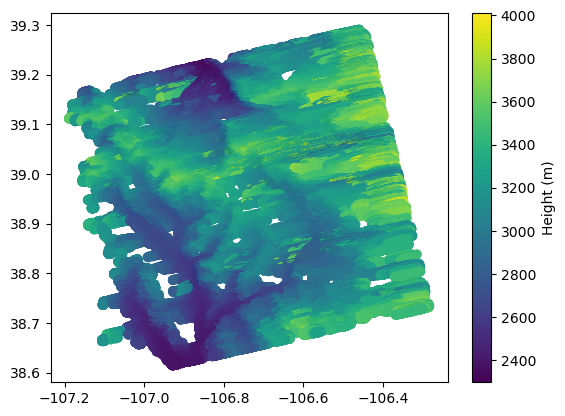
  azimuth_offset :

  3

Simple plot of the results

# This could take a few minutes to plot
plt.scatter(x=ds_PIXC.longitude, y=ds_PIXC.latitude, c=ds_PIXC.height)
plt.colorbar().set_label('Height (m)')

4. Water Mask Pixel Cloud Vector Attribute NetCDF

Search for data of interest

pixcvec_results = earthaccess.search_data(short_name = 'SWOT_L2_HR_PIXCVEC_2.0',
                                        #granule_name = '*_009_*', # pass number 9 if we want to filter further
                                        #temporal = ('2024-02-01 00:00:00', '2024-02-29 23:59:59'), # can also specify by time
                                        bounding_box = (-106.62, 38.809, -106.54, 38.859)) # Lake Travis near Austin, TX

Granules found: 19

Let’s download the first data file! earthaccess.download has a list as the input format, so we need to put brackets around the single file we pass.

earthaccess.download([pixcvec_results[0]], "./data_downloads")

 Getting 1 granules, approx download size: 0.21 GB

['SWOT_L2_HR_PIXCVec_007_106_086R_20231127T042024_20231127T042035_PIC0_04.nc']

Open data using xarray

First, we’ll programmatically get the filename we just downloaded and then view the file via xarray.

ds_PIXCVEC = xr.open_mfdataset("data_downloads/SWOT_L2_HR_PIXCVec_*.nc", decode_cf=False,  engine='h5netcdf')
ds_PIXCVEC

<xarray.Dataset>
Dimensions:               (points: 2831150, nchar_reach_id: 11,
                           nchar_node_id: 14, nchar_lake_id: 10,
                           nchar_obs_id: 13)
Dimensions without coordinates: points, nchar_reach_id, nchar_node_id,
                                nchar_lake_id, nchar_obs_id
Data variables:
    azimuth_index         (points) int32 dask.array<chunksize=(2831150,), meta=np.ndarray>
    range_index           (points) int32 dask.array<chunksize=(2831150,), meta=np.ndarray>
    latitude_vectorproc   (points) float64 dask.array<chunksize=(2831150,), meta=np.ndarray>
    longitude_vectorproc  (points) float64 dask.array<chunksize=(2831150,), meta=np.ndarray>
    height_vectorproc     (points) float32 dask.array<chunksize=(2831150,), meta=np.ndarray>
    reach_id              (points, nchar_reach_id) |S1 dask.array<chunksize=(2831150, 11), meta=np.ndarray>
    node_id               (points, nchar_node_id) |S1 dask.array<chunksize=(2831150, 14), meta=np.ndarray>
    lake_id               (points, nchar_lake_id) |S1 dask.array<chunksize=(2831150, 10), meta=np.ndarray>
    obs_id                (points, nchar_obs_id) |S1 dask.array<chunksize=(2831150, 13), meta=np.ndarray>
    ice_clim_f            (points) int8 dask.array<chunksize=(2831150,), meta=np.ndarray>
    ice_dyn_f             (points) int8 dask.array<chunksize=(2831150,), meta=np.ndarray>
Attributes: (12/45)
    Conventions:                     CF-1.7
    title:                           Level 2 KaRIn high rate pixel cloud vect...
    short_name:                      L2_HR_PIXCVec
    institution:                     CNES
    source:                          Level 1B KaRIn High Rate Single Look Com...
    history:                         2023-12-03T05:59:43.712142Z: Creation
    ...                              ...
    xref_prior_river_db_file:
    xref_prior_lake_db_file:         SWOT_LakeDatabase_Nom_106_20000101T00000...
    xref_reforbittrack_files:        SWOT_RefOrbitTrackTileBoundary_Nom_20000...
    xref_param_l2_hr_laketile_file:  SWOT_Param_L2_HR_LakeTile_20000101T00000...
    ellipsoid_semi_major_axis:       6378137.0
    ellipsoid_flattening:            0.0033528106647474805

xarray.Dataset

• Dimensions:
  • points: 2831150
  • nchar_reach_id: 11
  • nchar_node_id: 14
  • nchar_lake_id: 10
  • nchar_obs_id: 13
• Coordinates: (0)
• Data variables: (11)
  • azimuth_index
    (points)
    int32
    dask.array<chunksize=(2831150,), meta=np.ndarray>

    _FillValue :

    2147483647

    long_name :

    rare interferogram azimuth index

    units :

    1

    valid_min :

    0

    valid_max :

    999999

    coordinates :

    longitude_vectorproc latitude_vectorproc

    comment :

    Rare interferogram azimuth index (indexed from 0).

    Array Chunk Bytes 11.32 MB 11.32 MB Shape (2831150,) (2831150,) Count 2 Tasks 1 Chunks Type int32 numpy.ndarray

  • range_index
    (points)
    int32
    dask.array<chunksize=(2831150,), meta=np.ndarray>

    _FillValue :

    2147483647

    long_name :

    rare interferogram range index

    units :

    1

    valid_min :

    0

    valid_max :

    999999

    coordinates :

    longitude_vectorproc latitude_vectorproc

    comment :

    Rare interferogram range index (indexed from 0).

    Array Chunk Bytes 11.32 MB 11.32 MB Shape (2831150,) (2831150,) Count 2 Tasks 1 Chunks Type int32 numpy.ndarray

  • latitude_vectorproc
    (points)
    float64
    dask.array<chunksize=(2831150,), meta=np.ndarray>

    _FillValue :

    9.969209968386869e+36

    long_name :

    height-constrained geolocation latitude

    standard_name :

    latitude

    units :

    degrees_north

    valid_min :

    -80.0

    valid_max :

    80.0

    comment :

    Height-constrained geodetic latitude of the pixel. Units are in degrees north of the equator.

    Array Chunk Bytes 22.65 MB 22.65 MB Shape (2831150,) (2831150,) Count 2 Tasks 1 Chunks Type float64 numpy.ndarray

  • longitude_vectorproc
    (points)
    float64
    dask.array<chunksize=(2831150,), meta=np.ndarray>

    _FillValue :

    9.969209968386869e+36

    long_name :

    height-constrained geolocation longitude

    standard_name :

    longitude

    units :

    degrees_east

    valid_min :

    -180.0

    valid_max :

    180.0

    comment :

    Height-constrained geodetic longitude of the pixel. Positive=degrees east of the Greenwich meridian. Negative=degrees west of the Greenwich meridian.

    Array Chunk Bytes 22.65 MB 22.65 MB Shape (2831150,) (2831150,) Count 2 Tasks 1 Chunks Type float64 numpy.ndarray

  • height_vectorproc
    (points)
    float32
    dask.array<chunksize=(2831150,), meta=np.ndarray>

    _FillValue :

    9.96921e+36

    long_name :

    height above reference ellipsoid

    units :

    m

    valid_min :

    -1500.0

    valid_max :

    15000.0

    coordinates :

    longitude_vectorproc latitude_vectorproc

    comment :

    Height-constrained height of the pixel above the reference ellipsoid.

    Array Chunk Bytes 11.32 MB 11.32 MB Shape (2831150,) (2831150,) Count 2 Tasks 1 Chunks Type float32 numpy.ndarray

  • reach_id
    (points, nchar_reach_id)
    |S1
    dask.array<chunksize=(2831150, 11), meta=np.ndarray>

    long_name :

    identifier of the associated prior river reach

    coordinates :

    longitude_vectorproc latitude_vectorproc

    comment :

    Unique reach identifier from the prior river database. The format of the identifier is CBBBBBRRRRT, where C=continent, B=basin, R=reach, T=type.

    Array Chunk Bytes 31.14 MB 31.14 MB Shape (2831150, 11) (2831150, 11) Count 2 Tasks 1 Chunks Type |S1 numpy.ndarray

  • node_id
    (points, nchar_node_id)
    |S1
    dask.array<chunksize=(2831150, 14), meta=np.ndarray>

    long_name :

    identifier of the associated prior river node

    coordinates :

    longitude_vectorproc latitude_vectorproc

    comment :

    Unique node identifier from the prior river database. The format of the identifier is CBBBBBRRRRNNNT, where C=continent, B=basin, R=reach, N=node, T=type of water body.

    Array Chunk Bytes 39.64 MB 39.64 MB Shape (2831150, 14) (2831150, 14) Count 2 Tasks 1 Chunks Type |S1 numpy.ndarray

  • lake_id
    (points, nchar_lake_id)
    |S1
    dask.array<chunksize=(2831150, 10), meta=np.ndarray>

    long_name :

    identifier of the associated prior lake

    coordinates :

    longitude_vectorproc latitude_vectorproc

    comment :

    Identifier of the lake from the lake prior database) associated to the pixel. The format of the identifier is CBBNNNNNNT, where C=continent, B=basin, N=counter within the basin, T=type of water body.

    Array Chunk Bytes 28.31 MB 28.31 MB Shape (2831150, 10) (2831150, 10) Count 2 Tasks 1 Chunks Type |S1 numpy.ndarray

  • obs_id
    (points, nchar_obs_id)
    |S1
    dask.array<chunksize=(2831150, 13), meta=np.ndarray>

    long_name :

    identifier of the observed feature

    coordinates :

    longitude_vectorproc latitude_vectorproc

    comment :

    Tile-specific identifier of the observed feature associated to the pixel. The format of the identifier is CBBTTTSNNNNNN, where C=continent, B=basin, T=tile number, S=swath side, N=lake counter within the PIXC tile.

    Array Chunk Bytes 36.80 MB 36.80 MB Shape (2831150, 13) (2831150, 13) Count 2 Tasks 1 Chunks Type |S1 numpy.ndarray

  • ice_clim_f
    (points)
    int8
    dask.array<chunksize=(2831150,), meta=np.ndarray>

    _FillValue :

    127

    long_name :

    climatological ice cover flag

    flag_meanings :

    no_ice_cover uncertain_ice_cover full_ice_cover

    flag_values :

    [0 1 2]

    institution :

    University of North Carolina

    coordinates :

    longitude_vectorproc latitude_vectorproc

    comment :

    Climatological ice cover flag indicating whether the pixel is ice-covered on the day of the observation based on external climatological information (not the SWOT measurement). Values of 0, 1, and 2 indicate that the surface is not ice covered, may or may not be partially or fully ice covered, and fully ice covered, respectively. A value of 127 indicates that this flag is not available.

    Array Chunk Bytes 2.83 MB 2.83 MB Shape (2831150,) (2831150,) Count 2 Tasks 1 Chunks Type int8 numpy.ndarray

  • ice_dyn_f
    (points)
    int8
    dask.array<chunksize=(2831150,), meta=np.ndarray>

    _FillValue :

    127

    long_name :

    dynamical ice cover flag

    flag_meanings :

    no_ice_cover partial_ice_cover full_ice_cover

    flag_values :

    [0 1 2]

    institution :

    University of North Carolina

    coordinates :

    longitude_vectorproc latitude_vectorproc

    comment :

    Dynamic ice cover flag indicating whether the pixel is ice-covered on the day of the observation based on analysis of external satellite optical data. Values of 0, 1, and 2 indicate that the surface is not ice covered, partially ice covered, and fully ice covered, respectively. A value of 255 indicates that this flag is not available.

    Array Chunk Bytes 2.83 MB 2.83 MB Shape (2831150,) (2831150,) Count 2 Tasks 1 Chunks Type int8 numpy.ndarray

• Indexes: (0)
• Attributes: (45)

  Conventions :

  CF-1.7

  title :

  Level 2 KaRIn high rate pixel cloud vector attribute product

  short_name :

  L2_HR_PIXCVec

  institution :

  CNES

  source :

  Level 1B KaRIn High Rate Single Look Complex Data Product

  history :

  2023-12-03T05:59:43.712142Z: Creation

  platform :

  SWOT

  references :

  SWOT-DD-CDM-0565-CNES_SAS_Design_L2_HR_LakeSP - Revision A - 20220531

  reference_document :

  SWOT-TN-CDM-0677-CNES_Product_Description_L2_HR_PIXCVec - Revision A - 20220531

  product_version :

  V5.3.0

  crid :

  PIC0

  pge_name :

  PGE_L2_HR_LakeSP

  pge_version :

  V4.3.0

  contact :

  SWOT-contact@cnes.fr

  cycle_number :

  7

  pass_number :

  106

  tile_number :

  86

  swath_side :

  R

  tile_name :

  106_086R

  continent_id :

  NA

  continent_code :

  7

  time_granule_start :

  2023-11-27T04:20:24.437425Z

  time_granule_end :

  2023-11-27T04:20:35.530690Z

  time_coverage_start :

  2023-11-27T04:20:24Z

  time_coverage_end :

  2023-11-27T04:20:34.966118Z

  geospatial_lon_min :

  -107.2245094782927

  geospatial_lon_max :

  -106.32383090171766

  geospatial_lat_min :

  38.56164725058795

  geospatial_lat_max :

  39.320021843662694

  inner_first_longitude :

  -106.47881643041174

  inner_first_latitude :

  39.320021843662694

  inner_last_longitude :

  -106.32383090171766

  inner_last_latitude :

  38.69212711409543

  outer_first_longitude :

  -107.2245094782927

  outer_first_latitude :

  39.18406274086079

  outer_last_longitude :

  -107.04259075253788

  outer_last_latitude :

  38.56164725058795

  xref_l2_hr_pixc_file :

  SWOT_L2_HR_PIXC_007_106_086R_20231127T042024_20231127T042035_PIC0_03.nc

  xref_l2_hr_pixcvecriver_file :

  SWOT_L2_HR_PIXCVecRiver_007_106_086R_20231127T042024_20231127T042035_PIC0_04.nc

  xref_prior_river_db_file :

  xref_prior_lake_db_file :

  SWOT_LakeDatabase_Nom_106_20000101T000000_20991231T235959_20231017T000000_v105.sqlite

  xref_reforbittrack_files :

  SWOT_RefOrbitTrackTileBoundary_Nom_20000101T000000_21000101T000000_20200617T193054_v101.txt

  xref_param_l2_hr_laketile_file :

  SWOT_Param_L2_HR_LakeTile_20000101T000000_20991231T235959_20230922T160000_v411.cfg

  ellipsoid_semi_major_axis :

  6378137.0

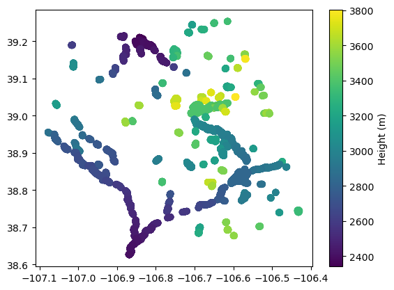
  ellipsoid_flattening :

  0.0033528106647474805

Simple plot

pixcvec_htvals = ds_PIXCVEC.height_vectorproc.compute()
pixcvec_latvals = ds_PIXCVEC.latitude_vectorproc.compute()
pixcvec_lonvals = ds_PIXCVEC.longitude_vectorproc.compute()

#Before plotting, we set all fill values to nan so that the graph shows up better spatially
pixcvec_htvals[pixcvec_htvals > 15000] = np.nan
pixcvec_latvals[pixcvec_latvals < 1] = np.nan
pixcvec_lonvals[pixcvec_lonvals > -1] = np.nan

plt.scatter(x=pixcvec_lonvals, y=pixcvec_latvals, c=pixcvec_htvals)
plt.colorbar().set_label('Height (m)')

5. Raster NetCDF

Search for data of interest

raster_results = earthaccess.search_data(short_name = 'SWOT_L2_HR_Raster_2.0',
                                        #temporal = ('2024-02-01 00:00:00', '2024-02-29 23:59:59'), # can also specify by time
                                        granule_name = '*100m*', # here we filter by files with '100m' in the name (This collection has two resolution options: 100m & 250m)
                                        bounding_box = (-106.62, 38.809, -106.54, 38.859)) # Lake Travis near Austin, TX

Granules found: 34

Let’s download one data file.

earthaccess.download([raster_results[0]], "./data_downloads")

 Getting 1 granules, approx download size: 0.04 GB

['SWOT_L2_HR_Raster_100m_UTM13S_N_x_x_x_007_106_043F_20231127T042014_20231127T042035_PIC0_04.nc']

Open data with xarray

First, we’ll programmatically get the filename we just downloaded and then view the file via xarray.

ds_raster = xr.open_mfdataset(f'data_downloads/SWOT_L2_HR_Raster*', engine='h5netcdf')
ds_raster

<xarray.Dataset>
Dimensions:                  (x: 1520, y: 1519)
Coordinates:
  * x                        (x) float64 2.969e+05 2.97e+05 ... 4.488e+05
  * y                        (y) float64 4.274e+06 4.274e+06 ... 4.426e+06
Data variables: (12/39)
    crs                      object ...
    longitude                (y, x) float64 dask.array<chunksize=(1519, 1520), meta=np.ndarray>
    latitude                 (y, x) float64 dask.array<chunksize=(1519, 1520), meta=np.ndarray>
    wse                      (y, x) float32 dask.array<chunksize=(1519, 1520), meta=np.ndarray>
    wse_qual                 (y, x) float32 dask.array<chunksize=(1519, 1520), meta=np.ndarray>
    wse_qual_bitwise         (y, x) float64 dask.array<chunksize=(1519, 1520), meta=np.ndarray>
    ...                       ...
    load_tide_fes            (y, x) float32 dask.array<chunksize=(1519, 1520), meta=np.ndarray>
    load_tide_got            (y, x) float32 dask.array<chunksize=(1519, 1520), meta=np.ndarray>
    pole_tide                (y, x) float32 dask.array<chunksize=(1519, 1520), meta=np.ndarray>
    model_dry_tropo_cor      (y, x) float32 dask.array<chunksize=(1519, 1520), meta=np.ndarray>
    model_wet_tropo_cor      (y, x) float32 dask.array<chunksize=(1519, 1520), meta=np.ndarray>
    iono_cor_gim_ka          (y, x) float32 dask.array<chunksize=(1519, 1520), meta=np.ndarray>
Attributes: (12/49)
    Conventions:                   CF-1.7
    title:                         Level 2 KaRIn High Rate Raster Data Product
    source:                        Ka-band radar interferometer
    history:                       2023-12-03T08:26:57Z : Creation
    platform:                      SWOT
    references:                    V1.1.1
    ...                            ...
    x_min:                         296900.0
    x_max:                         448800.0
    y_min:                         4274000.0
    y_max:                         4425800.0
    institution:                   CNES
    product_version:               04

xarray.Dataset

• Dimensions:
  • x: 1520
  • y: 1519
• Coordinates: (2)
  • x
    (x)
    float64
    2.969e+05 2.97e+05 ... 4.488e+05

    long_name :

    x coordinate of projection

    standard_name :

    projection_x_coordinate

    units :

    m

    valid_min :

    -10000000.0

    valid_max :

    10000000.0

    comment :

    UTM easting coordinate of the pixel.

    array([296900., 297000., 297100., ..., 448600., 448700., 448800.])

  • y
    (y)
    float64
    4.274e+06 4.274e+06 ... 4.426e+06

    long_name :

    y coordinate of projection

    standard_name :

    projection_y_coordinate

    units :

    m

    valid_min :

    -20000000.0

    valid_max :

    20000000.0

    comment :

    UTM northing coordinate of the pixel.

    array([4274000., 4274100., 4274200., ..., 4425600., 4425700., 4425800.])

• Data variables: (39)
  • crs
    ()
    object
    ...

    long_name :

    CRS Definition

    grid_mapping_name :

    transverse_mercator

    projected_crs_name :

    WGS 84 / UTM zone 13N

    geographic_crs_name :

    WGS 84

    reference_ellipsoid_name :

    WGS 84

    horizontal_datum_name :

    WGS_1984

    prime_meridian_name :

    Greenwich

    false_easting :

    500000.0

    false_northing :

    0.0

    longitude_of_central_meridian :

    -105.0

    longitude_of_prime_meridian :

    0.0

    latitude_of_projection_origin :

    0.0

    scale_factor_at_central_meridian :

    0.9996

    semi_major_axis :

    6378137.0

    inverse_flattening :

    298.257223563

    crs_wkt :

    PROJCS["WGS 84 / UTM zone 13N",GEOGCS["WGS 84",DATUM["WGS_1984",SPHEROID["WGS 84",6378137,298.257223563,AUTHORITY["EPSG","7030"]],AUTHORITY["EPSG","6326"]],PRIMEM["Greenwich",0,AUTHORITY["EPSG","8901"]],UNIT["degree",0.0174532925199433,AUTHORITY["EPSG","9122"]],AUTHORITY["EPSG","4326"]],PROJECTION["Transverse_Mercator"],PARAMETER["latitude_of_origin",0],PARAMETER["central_meridian",-105],PARAMETER["scale_factor",0.9996],PARAMETER["false_easting",500000],PARAMETER["false_northing",0],UNIT["metre",1,AUTHORITY["EPSG","9001"]],AXIS["Easting",EAST],AXIS["Northing",NORTH],AUTHORITY["EPSG","32613"]]

    spatial_ref :

    PROJCS["WGS 84 / UTM zone 13N",GEOGCS["WGS 84",DATUM["WGS_1984",SPHEROID["WGS 84",6378137,298.257223563,AUTHORITY["EPSG","7030"]],AUTHORITY["EPSG","6326"]],PRIMEM["Greenwich",0,AUTHORITY["EPSG","8901"]],UNIT["degree",0.0174532925199433,AUTHORITY["EPSG","9122"]],AUTHORITY["EPSG","4326"]],PROJECTION["Transverse_Mercator"],PARAMETER["latitude_of_origin",0],PARAMETER["central_meridian",-105],PARAMETER["scale_factor",0.9996],PARAMETER["false_easting",500000],PARAMETER["false_northing",0],UNIT["metre",1,AUTHORITY["EPSG","9001"]],AXIS["Easting",EAST],AXIS["Northing",NORTH],AUTHORITY["EPSG","32613"]]

    comment :

    UTM zone coordinate reference system.

    [1 values with dtype=object]

  • longitude
    (y, x)
    float64
    dask.array<chunksize=(1519, 1520), meta=np.ndarray>

    long_name :

    longitude (degrees East)

    standard_name :

    longitude

    grid_mapping :

    crs

    units :

    degrees_east

    valid_min :

    -180.0

    valid_max :

    180.0

    comment :

    Geodetic longitude [-180,180) (east of the Greenwich meridian) of the pixel.

    Array Chunk Bytes 18.47 MB 18.47 MB Shape (1519, 1520) (1519, 1520) Count 2 Tasks 1 Chunks Type float64 numpy.ndarray

  • latitude
    (y, x)
    float64
    dask.array<chunksize=(1519, 1520), meta=np.ndarray>

    long_name :

    latitude (positive N, negative S)

    standard_name :

    latitude

    grid_mapping :

    crs

    units :

    degrees_north

    valid_min :

    -80.0

    valid_max :

    80.0

    comment :

    Geodetic latitude [-80,80] (degrees north of equator) of the pixel.

    Array Chunk Bytes 18.47 MB 18.47 MB Shape (1519, 1520) (1519, 1520) Count 2 Tasks 1 Chunks Type float64 numpy.ndarray

  • wse
    (y, x)
    float32
    dask.array<chunksize=(1519, 1520), meta=np.ndarray>

    long_name :

    water surface elevation above geoid

    grid_mapping :

    crs

    units :

    m

    quality_flag :

    wse_qual

    valid_min :

    -1500.0

    valid_max :

    15000.0

    comment :

    Water surface elevation of the pixel above the geoid and after using models to subtract the effects of tides (solid_earth_tide, load_tide_fes, pole_tide).

    Array Chunk Bytes 9.24 MB 9.24 MB Shape (1519, 1520) (1519, 1520) Count 2 Tasks 1 Chunks Type float32 numpy.ndarray

  • wse_qual
    (y, x)
    float32
    dask.array<chunksize=(1519, 1520), meta=np.ndarray>

    long_name :

    summary quality indicator for the water surface elevation

    standard_name :

    status_flag

    grid_mapping :

    crs

    flag_meanings :

    good suspect degraded bad

    flag_values :

    [0 1 2 3]

    valid_min :

    0

    valid_max :

    3

    comment :

    Summary quality indicator for the water surface elevation quantities. A value of 0 indicates a nominal measurement, 1 indicates a suspect measurement, 2 indicates a degraded measurement, and 3 indicates a bad measurement.

    Array Chunk Bytes 9.24 MB 9.24 MB Shape (1519, 1520) (1519, 1520) Count 2 Tasks 1 Chunks Type float32 numpy.ndarray

  • wse_qual_bitwise
    (y, x)
    float64
    dask.array<chunksize=(1519, 1520), meta=np.ndarray>

    long_name :

    bitwise quality indicator for the water surface elevation

    standard_name :

    status_flag

    grid_mapping :

    crs

    flag_meanings :

    classification_qual_suspect geolocation_qual_suspect large_uncert_suspect bright_land few_pixels far_range_suspect near_range_suspect classification_qual_degraded geolocation_qual_degraded low_coherence_water_degraded value_bad no_pixels outside_scene_bounds inner_swath missing_karin_data

    flag_masks :

    [ 2 4 32 128 4096 8192 16384 262144 524288 2097152 16777216 268435456 536870912 1073741824 2147483648]

    valid_min :

    0

    valid_max :

    4046221478

    comment :

    Bitwise quality indicator for the water surface elevation quantities. If this word is interpreted as an unsigned integer, a value of 0 indicates good data, positive values less than 32768 represent suspect data, values greater than or equal to 32768 but less than 8388608 represent degraded data, and values greater than or equal to 8388608 represent bad data.

    Array Chunk Bytes 18.47 MB 18.47 MB Shape (1519, 1520) (1519, 1520) Count 2 Tasks 1 Chunks Type float64 numpy.ndarray

  • wse_uncert
    (y, x)
    float32
    dask.array<chunksize=(1519, 1520), meta=np.ndarray>

    long_name :

    uncertainty in the water surface elevation

    grid_mapping :

    crs

    units :

    m

    valid_min :

    0.0

    valid_max :

    999999.0

    comment :

    1-sigma uncertainty in the water surface elevation.

    Array Chunk Bytes 9.24 MB 9.24 MB Shape (1519, 1520) (1519, 1520) Count 2 Tasks 1 Chunks Type float32 numpy.ndarray

  • water_area
    (y, x)
    float32
    dask.array<chunksize=(1519, 1520), meta=np.ndarray>

    long_name :

    water surface area

    grid_mapping :

    crs

    units :

    m^2

    quality_flag :

    water_area_qual

    valid_min :

    -2000000.0

    valid_max :

    2000000000.0

    comment :

    Surface area of the water pixels.

    Array Chunk Bytes 9.24 MB 9.24 MB Shape (1519, 1520) (1519, 1520) Count 2 Tasks 1 Chunks Type float32 numpy.ndarray

  • water_area_qual
    (y, x)
    float32
    dask.array<chunksize=(1519, 1520), meta=np.ndarray>

    long_name :

    summary quality indicator for the water surface area

    standard_name :

    status_flag

    grid_mapping :

    crs

    flag_meanings :

    good suspect degraded bad

    flag_values :

    [0 1 2 3]

    valid_min :

    0

    valid_max :

    3

    comment :

    Summary quality indicator for the water surface area and water fraction quantities. A value of 0 indicates a nominal measurement, 1 indicates a suspect measurement, 2 indicates a degraded measurement, and 3 indicates a bad measurement.

    Array Chunk Bytes 9.24 MB 9.24 MB Shape (1519, 1520) (1519, 1520) Count 2 Tasks 1 Chunks Type float32 numpy.ndarray

  • water_area_qual_bitwise
    (y, x)
    float64
    dask.array<chunksize=(1519, 1520), meta=np.ndarray>

    long_name :

    bitwise quality indicator for the water surface area

    standard_name :

    status_flag

    grid_mapping :

    crs

    flag_meanings :

    classification_qual_suspect geolocation_qual_suspect water_fraction_suspect large_uncert_suspect bright_land low_coherence_water_suspect few_pixels far_range_suspect near_range_suspect classification_qual_degraded geolocation_qual_degraded value_bad no_pixels outside_scene_bounds inner_swath missing_karin_data

    flag_masks :

    [ 2 4 8 32 128 256 4096 8192 16384 262144 524288 16777216 268435456 536870912 1073741824 2147483648]

    valid_min :

    0

    valid_max :

    4044124590

    comment :

    Bitwise quality indicator for the water surface area and water fraction quantities. If this word is interpreted as an unsigned integer, a value of 0 indicates good data, positive values less than 32768 represent suspect data, values greater than or equal to 32768 but less than 8388608 represent degraded data, and values greater than or equal to 8388608 represent bad data.

    Array Chunk Bytes 18.47 MB 18.47 MB Shape (1519, 1520) (1519, 1520) Count 2 Tasks 1 Chunks Type float64 numpy.ndarray

  • water_area_uncert
    (y, x)
    float32
    dask.array<chunksize=(1519, 1520), meta=np.ndarray>

    long_name :

    uncertainty in the water surface area

    grid_mapping :

    crs

    units :

    m^2

    valid_min :

    0.0

    valid_max :

    2000000000.0

    comment :

    1-sigma uncertainty in the water surface area.

    Array Chunk Bytes 9.24 MB 9.24 MB Shape (1519, 1520) (1519, 1520) Count 2 Tasks 1 Chunks Type float32 numpy.ndarray

  • water_frac
    (y, x)
    float32
    dask.array<chunksize=(1519, 1520), meta=np.ndarray>

    long_name :

    water fraction

    grid_mapping :

    crs

    units :

    1

    quality_flag :

    water_area_qual

    valid_min :

    -1000.0

    valid_max :

    10000.0

    comment :

    Fraction of the pixel that is water.

    Array Chunk Bytes 9.24 MB 9.24 MB Shape (1519, 1520) (1519, 1520) Count 2 Tasks 1 Chunks Type float32 numpy.ndarray

  • water_frac_uncert
    (y, x)
    float32
    dask.array<chunksize=(1519, 1520), meta=np.ndarray>

    long_name :

    uncertainty in the water fraction

    grid_mapping :

    crs

    units :

    1

    valid_min :

    0.0

    valid_max :

    999999.0

    comment :

    1-sigma uncertainty in the water fraction.

    Array Chunk Bytes 9.24 MB 9.24 MB Shape (1519, 1520) (1519, 1520) Count 2 Tasks 1 Chunks Type float32 numpy.ndarray

  • sig0
    (y, x)
    float32
    dask.array<chunksize=(1519, 1520), meta=np.ndarray>

    long_name :

    sigma0

    grid_mapping :

    crs

    units :

    1

    quality_flag :

    sig0_qual

    valid_min :

    -1000.0

    valid_max :

    10000000.0

    comment :

    Normalized radar cross section (sigma0) in real, linear units (not decibels). The value may be negative due to noise subtraction.

    Array Chunk Bytes 9.24 MB 9.24 MB Shape (1519, 1520) (1519, 1520) Count 2 Tasks 1 Chunks Type float32 numpy.ndarray

  • sig0_qual
    (y, x)
    float32
    dask.array<chunksize=(1519, 1520), meta=np.ndarray>

    long_name :

    summary quality indicator for the sigma0

    standard_name :

    status_flag

    grid_mapping :

    crs

    flag_meanings :

    good suspect degraded bad

    flag_values :

    [0 1 2 3]

    valid_min :

    0

    valid_max :

    3

    comment :

    Summary quality indicator for the sigma0 quantities. A value of 0 indicates a nominal measurement, 1 indicates a suspect measurement, 2 indicates a degraded measurement, and 3 indicates a bad measurement.

    Array Chunk Bytes 9.24 MB 9.24 MB Shape (1519, 1520) (1519, 1520) Count 2 Tasks 1 Chunks Type float32 numpy.ndarray

  • sig0_qual_bitwise
    (y, x)
    float64
    dask.array<chunksize=(1519, 1520), meta=np.ndarray>

    long_name :

    bitwise quality indicator for the sigma0

    standard_name :

    status_flag

    grid_mapping :

    crs

    flag_meanings :

    sig0_qual_suspect classification_qual_suspect geolocation_qual_suspect large_uncert_suspect bright_land low_coherence_water_suspect few_pixels far_range_suspect near_range_suspect sig0_qual_degraded classification_qual_degraded geolocation_qual_degraded value_bad no_pixels outside_scene_bounds inner_swath missing_karin_data

    flag_masks :

    [ 1 2 4 32 128 256 4096 8192 16384 131072 262144 524288 16777216 268435456 536870912 1073741824 2147483648]

    valid_min :

    0

    valid_max :

    4044255655

    comment :

    Bitwise quality indicator for the sigma0 quantities. If this word is interpreted as an unsigned integer, a value of 0 indicates good data, positive values less than 32768 represent suspect data, values greater than or equal to 32768 but less than 8388608 represent degraded data, and values greater than or equal to 8388608 represent bad data.

    Array Chunk Bytes 18.47 MB 18.47 MB Shape (1519, 1520) (1519, 1520) Count 2 Tasks 1 Chunks Type float64 numpy.ndarray

  • sig0_uncert
    (y, x)
    float32
    dask.array<chunksize=(1519, 1520), meta=np.ndarray>

    long_name :

    uncertainty in sigma0

    grid_mapping :

    crs

    units :

    1

    valid_min :

    0.0

    valid_max :

    1000.0

    comment :

    1-sigma uncertainty in sigma0. The value is provided in linear units. This value is a one-sigma additive (not multiplicative) uncertainty term, which can be added to or subtracted from sigma0.

    Array Chunk Bytes 9.24 MB 9.24 MB Shape (1519, 1520) (1519, 1520) Count 2 Tasks 1 Chunks Type float32 numpy.ndarray

  • inc
    (y, x)
    float32
    dask.array<chunksize=(1519, 1520), meta=np.ndarray>

    long_name :

    incidence angle

    grid_mapping :

    crs

    units :

    degrees

    valid_min :

    0.0

    valid_max :

    90.0

    comment :

    Incidence angle.

    Array Chunk Bytes 9.24 MB 9.24 MB Shape (1519, 1520) (1519, 1520) Count 2 Tasks 1 Chunks Type float32 numpy.ndarray

  • cross_track
    (y, x)
    float32
    dask.array<chunksize=(1519, 1520), meta=np.ndarray>

    long_name :

    approximate cross-track location

    grid_mapping :

    crs

    units :

    m

    valid_min :

    -75000.0

    valid_max :

    75000.0

    comment :

    Approximate cross-track location of the pixel.

    Array Chunk Bytes 9.24 MB 9.24 MB Shape (1519, 1520) (1519, 1520) Count 2 Tasks 1 Chunks Type float32 numpy.ndarray

  • illumination_time
    (y, x)
    datetime64[ns]
    dask.array<chunksize=(1519, 1520), meta=np.ndarray>

    long_name :

    time of illumination of each pixel (UTC)

    standard_name :

    time

    tai_utc_difference :

    37.0

    leap_second :

    0000-00-00T00:00:00Z

    comment :

    Time of measurement in seconds in the UTC time scale since 1 Jan 2000 00:00:00 UTC. [tai_utc_difference] is the difference between TAI and UTC reference time (seconds) for the first measurement of the data set. If a leap second occurs within the data set, the attribute leap_second is set to the UTC time at which the leap second occurs.

    Array Chunk Bytes 18.47 MB 18.47 MB Shape (1519, 1520) (1519, 1520) Count 2 Tasks 1 Chunks Type datetime64[ns] numpy.ndarray

  • illumination_time_tai
    (y, x)
    datetime64[ns]
    dask.array<chunksize=(1519, 1520), meta=np.ndarray>

    long_name :

    time of illumination of each pixel (TAI)

    standard_name :

    time

    comment :

    Time of measurement in seconds in the TAI time scale since 1 Jan 2000 00:00:00 TAI. This time scale contains no leap seconds. The difference (in seconds) with time in UTC is given by the attribute [illumination_time:tai_utc_difference].

    Array Chunk Bytes 18.47 MB 18.47 MB Shape (1519, 1520) (1519, 1520) Count 2 Tasks 1 Chunks Type datetime64[ns] numpy.ndarray

  • n_wse_pix
    (y, x)
    float64
    dask.array<chunksize=(1519, 1520), meta=np.ndarray>

    long_name :

    number of water surface elevation pixels

    grid_mapping :

    crs

    units :

    l

    valid_min :

    0

    valid_max :

    999999

    comment :

    Number of pixel cloud samples used in water surface elevation aggregation.

    Array Chunk Bytes 18.47 MB 18.47 MB Shape (1519, 1520) (1519, 1520) Count 2 Tasks 1 Chunks Type float64 numpy.ndarray

  • n_water_area_pix
    (y, x)
    float64
    dask.array<chunksize=(1519, 1520), meta=np.ndarray>

    long_name :

    number of water surface area pixels

    grid_mapping :

    crs

    units :

    l

    valid_min :

    0

    valid_max :

    999999

    comment :

    Number of pixel cloud samples used in water surface area and water fraction aggregation.

    Array Chunk Bytes 18.47 MB 18.47 MB Shape (1519, 1520) (1519, 1520) Count 2 Tasks 1 Chunks Type float64 numpy.ndarray

  • n_sig0_pix
    (y, x)
    float64
    dask.array<chunksize=(1519, 1520), meta=np.ndarray>

    long_name :

    number of sigma0 pixels

    grid_mapping :

    crs

    units :

    l

    valid_min :

    0

    valid_max :

    999999

    comment :

    Number of pixel cloud samples used in sigma0 aggregation.

    Array Chunk Bytes 18.47 MB 18.47 MB Shape (1519, 1520) (1519, 1520) Count 2 Tasks 1 Chunks Type float64 numpy.ndarray

  • n_other_pix
    (y, x)
    float64
    dask.array<chunksize=(1519, 1520), meta=np.ndarray>

    long_name :

    number of other pixels

    grid_mapping :

    crs

    units :

    l

    valid_min :

    0

    valid_max :

    999999

    comment :

    Number of pixel cloud samples used in aggregation of quantities not related to water surface elevation, water surface area, water fraction or sigma0.

    Array Chunk Bytes 18.47 MB 18.47 MB Shape (1519, 1520) (1519, 1520) Count 2 Tasks 1 Chunks Type float64 numpy.ndarray

  • dark_frac
    (y, x)
    float32
    dask.array<chunksize=(1519, 1520), meta=np.ndarray>

    long_name :

    fractional area of dark water

    grid_mapping :

    crs

    units :

    l

    valid_min :

    -1000.0

    valid_max :

    10000.0

    comment :

    Fraction of pixel water surface area covered by dark water.

    Array Chunk Bytes 9.24 MB 9.24 MB Shape (1519, 1520) (1519, 1520) Count 2 Tasks 1 Chunks Type float32 numpy.ndarray

  • ice_clim_flag
    (y, x)
    float32
    dask.array<chunksize=(1519, 1520), meta=np.ndarray>

    long_name :

    climatological ice cover flag

    standard_name :

    status_flag

    source :

    UNC

    grid_mapping :

    crs

    flag_meanings :

    no_ice_cover uncertain_ice_cover full_ice_cover

    flag_values :

    [0 1 2]

    valid_min :

    0

    valid_max :

    2

    comment :

    Climatological ice cover flag indicating whether the pixel is ice-covered on the day of the observation based on external climatological information (not the SWOT measurement). Values of 0, 1, and 2 indicate that the pixel is likely not ice covered, may or may not be partially or fully ice covered, and likely fully ice covered, respectively.

    Array Chunk Bytes 9.24 MB 9.24 MB Shape (1519, 1520) (1519, 1520) Count 2 Tasks 1 Chunks Type float32 numpy.ndarray

  • ice_dyn_flag
    (y, x)
    float32
    dask.array<chunksize=(1519, 1520), meta=np.ndarray>

    long_name :

    dynamic ice cover flag

    standard_name :

    status_flag

    source :

    UNC

    grid_mapping :

    crs

    flag_meanings :

    no_ice_cover partial_ice_cover full_ice_cover

    flag_values :

    [0 1 2]

    valid_min :

    0

    valid_max :

    2

    comment :

    Dynamic ice cover flag indicating whether the surface is ice-covered on the day of the observation based on analysis of external satellite optical data. Values of 0, 1, and 2 indicate that the pixel is not ice covered, partially ice covered, and fully ice covered, respectively.

    Array Chunk Bytes 9.24 MB 9.24 MB Shape (1519, 1520) (1519, 1520) Count 2 Tasks 1 Chunks Type float32 numpy.ndarray

  • layover_impact
    (y, x)
    float32
    dask.array<chunksize=(1519, 1520), meta=np.ndarray>

    long_name :

    layover impact

    grid_mapping :

    crs

    units :

    m

    valid_min :

    -999999.0

    valid_max :

    999999.0

    comment :

    Estimate of the water surface elevation error caused by layover.

    Array Chunk Bytes 9.24 MB 9.24 MB Shape (1519, 1520) (1519, 1520) Count 2 Tasks 1 Chunks Type float32 numpy.ndarray

  • sig0_cor_atmos_model
    (y, x)
    float32
    dask.array<chunksize=(1519, 1520), meta=np.ndarray>

    long_name :

    two-way atmospheric correction to sigma0 from model

    source :

    European Centre for Medium-Range Weather Forecasts

    institution :

    ECMWF

    grid_mapping :

    crs

    units :

    1

    valid_min :

    1.0

    valid_max :

    10.0

    comment :

    Atmospheric correction to sigma0 from weather model data as a linear power multiplier (not decibels). sig0_cor_atmos_model is already applied in computing sig0.

    Array Chunk Bytes 9.24 MB 9.24 MB Shape (1519, 1520) (1519, 1520) Count 2 Tasks 1 Chunks Type float32 numpy.ndarray

  • height_cor_xover
    (y, x)
    float32
    dask.array<chunksize=(1519, 1520), meta=np.ndarray>

    long_name :

    height correction from KaRIn crossovers

    grid_mapping :

    crs

    units :

    m

    valid_min :

    -10.0

    valid_max :

    10.0

    comment :

    Height correction from KaRIn crossover calibration. The correction is applied before geolocation but reported as an equivalent height correction.

    Array Chunk Bytes 9.24 MB 9.24 MB Shape (1519, 1520) (1519, 1520) Count 2 Tasks 1 Chunks Type float32 numpy.ndarray

  • geoid
    (y, x)
    float32
    dask.array<chunksize=(1519, 1520), meta=np.ndarray>

    long_name :

    geoid height

    standard_name :

    geoid_height_above_reference_ellipsoid

    source :

    EGM2008 (Pavlis et al., 2012)

    grid_mapping :

    crs

    units :

    m

    valid_min :

    -150.0

    valid_max :

    150.0

    comment :

    Geoid height above the reference ellipsoid with a correction to refer the value to the mean tide system, i.e. includes the permanent tide (zero frequency).

    Array Chunk Bytes 9.24 MB 9.24 MB Shape (1519, 1520) (1519, 1520) Count 2 Tasks 1 Chunks Type float32 numpy.ndarray

  • solid_earth_tide
    (y, x)
    float32
    dask.array<chunksize=(1519, 1520), meta=np.ndarray>

    long_name :

    solid Earth tide height

    source :

    Cartwright and Taylor (1971) and Cartwright and Edden (1973)

    grid_mapping :

    crs

    units :

    m

    valid_min :

    -1.0

    valid_max :

    1.0

    comment :

    Solid-Earth (body) tide height. The zero-frequency permanent tide component is not included.

    Array Chunk Bytes 9.24 MB 9.24 MB Shape (1519, 1520) (1519, 1520) Count 2 Tasks 1 Chunks Type float32 numpy.ndarray

  • load_tide_fes
    (y, x)
    float32
    dask.array<chunksize=(1519, 1520), meta=np.ndarray>

    long_name :

    geocentric load tide height (FES)

    source :

    FES2014b (Carrere et al., 2016)

    institution :

    LEGOS/CNES

    grid_mapping :

    crs

    units :

    m

    valid_min :

    -0.2

    valid_max :

    0.2

    comment :

    Geocentric load tide height. The effect of the ocean tide loading of the Earth’s crust.

    Array Chunk Bytes 9.24 MB 9.24 MB Shape (1519, 1520) (1519, 1520) Count 2 Tasks 1 Chunks Type float32 numpy.ndarray

  • load_tide_got
    (y, x)
    float32
    dask.array<chunksize=(1519, 1520), meta=np.ndarray>

    long_name :

    geocentric load tide height (GOT)

    source :

    GOT4.10c (Ray, 2013)

    institution :

    GSFC

    grid_mapping :

    crs

    units :

    m

    valid_min :

    -0.2

    valid_max :

    0.2

    comment :

    Geocentric load tide height. The effect of the ocean tide loading of the Earth’s crust. This value is reported for reference but is not applied to the reported height.

    Array Chunk Bytes 9.24 MB 9.24 MB Shape (1519, 1520) (1519, 1520) Count 2 Tasks 1 Chunks Type float32 numpy.ndarray

  • pole_tide
    (y, x)
    float32
    dask.array<chunksize=(1519, 1520), meta=np.ndarray>

    long_name :

    geocentric pole tide height

    source :

    Wahr (1985) and Desai et al. (2015)

    grid_mapping :

    crs

    units :

    m

    valid_min :

    -0.2

    valid_max :

    0.2

    comment :

    Geocentric pole tide height. The total of the contribution from the solid-Earth (body) pole tide height and the load pole tide height (i.e., the effect of the ocean pole tide loading of the Earth’s crust).

    Array Chunk Bytes 9.24 MB 9.24 MB Shape (1519, 1520) (1519, 1520) Count 2 Tasks 1 Chunks Type float32 numpy.ndarray

  • model_dry_tropo_cor
    (y, x)
    float32
    dask.array<chunksize=(1519, 1520), meta=np.ndarray>

    long_name :

    dry troposphere vertical correction

    source :

    European Centre for Medium-Range Weather Forecasts

    institution :

    ECMWF

    grid_mapping :

    crs

    units :

    m

    valid_min :

    -3.0

    valid_max :

    -1.5

    comment :

    Equivalent vertical correction due to dry troposphere delay. The reported water surface elevation, latitude and longitude are computed after adding negative media corrections to uncorrected range along slant-range paths, accounting for the differential delay between the two KaRIn antennas. The equivalent vertical correction is computed by applying obliquity factors to the slant-path correction. Adding the reported correction to the reported water surface elevation results in the uncorrected pixel height.

    Array Chunk Bytes 9.24 MB 9.24 MB Shape (1519, 1520) (1519, 1520) Count 2 Tasks 1 Chunks Type float32 numpy.ndarray

  • model_wet_tropo_cor
    (y, x)
    float32
    dask.array<chunksize=(1519, 1520), meta=np.ndarray>

    long_name :

    wet troposphere vertical correction

    source :

    European Centre for Medium-Range Weather Forecasts

    institution :

    ECMWF

    grid_mapping :

    crs

    units :

    m

    valid_min :

    -1.0

    valid_max :

    0.0

    comment :

    Equivalent vertical correction due to wet troposphere delay. The reported water surface elevation, latitude and longitude are computed after adding negative media corrections to uncorrected range along slant-range paths, accounting for the differential delay between the two KaRIn antennas. The equivalent vertical correction is computed by applying obliquity factors to the slant-path correction. Adding the reported correction to the reported water surface elevation results in the uncorrected pixel height.

    Array Chunk Bytes 9.24 MB 9.24 MB Shape (1519, 1520) (1519, 1520) Count 2 Tasks 1 Chunks Type float32 numpy.ndarray

  • iono_cor_gim_ka
    (y, x)
    float32
    dask.array<chunksize=(1519, 1520), meta=np.ndarray>

    long_name :

    ionosphere vertical correction

    source :

    Global Ionosphere Maps

    institution :

    JPL

    grid_mapping :

    crs

    units :

    m

    valid_min :

    -0.5

    valid_max :

    0.0

    comment :

    Equivalent vertical correction due to ionosphere delay. The reported water surface elevation, latitude and longitude are computed after adding negative media corrections to uncorrected range along slant-range paths, accounting for the differential delay between the two KaRIn antennas. The equivalent vertical correction is computed by applying obliquity factors to the slant-path correction. Adding the reported correction to the reported water surface elevation results in the uncorrected pixel height.

    Array Chunk Bytes 9.24 MB 9.24 MB Shape (1519, 1520) (1519, 1520) Count 2 Tasks 1 Chunks Type float32 numpy.ndarray

• Indexes: (2)
  • x
    PandasIndex

    PandasIndex(Float64Index([296900.0, 297000.0, 297100.0, 297200.0, 297300.0, 297400.0,
                  297500.0, 297600.0, 297700.0, 297800.0,
                  ...
                  447900.0, 448000.0, 448100.0, 448200.0, 448300.0, 448400.0,
                  448500.0, 448600.0, 448700.0, 448800.0],
                 dtype='float64', name='x', length=1520))

  • y
    PandasIndex

    PandasIndex(Float64Index([4274000.0, 4274100.0, 4274200.0, 4274300.0, 4274400.0, 4274500.0,
                  4274600.0, 4274700.0, 4274800.0, 4274900.0,
                  ...
                  4424900.0, 4425000.0, 4425100.0, 4425200.0, 4425300.0, 4425400.0,
                  4425500.0, 4425600.0, 4425700.0, 4425800.0],
                 dtype='float64', name='y', length=1519))

• Attributes: (49)

  Conventions :

  CF-1.7

  title :

  Level 2 KaRIn High Rate Raster Data Product

  source :

  Ka-band radar interferometer

  history :

  2023-12-03T08:26:57Z : Creation

  platform :

  SWOT

  references :

  V1.1.1

  reference_document :

  JPL D-56416 - Revision B - August 17, 2023

  contact :

  alexander.t.corben[at]jpl.nasa.gov

  cycle_number :

  7

  pass_number :

  106

  scene_number :

  43

  tile_numbers :

  [84 85 86 87 84 85 86 87]

  tile_names :

  106_084L, 106_085L, 106_086L, 106_087L, 106_084R, 106_085R, 106_086R, 106_087R

  tile_polarizations :

  V, V, V, V, H, H, H, H

  coordinate_reference_system :

  Universal Transverse Mercator

  resolution :

  100.0

  short_name :

  L2_HR_Raster

  descriptor_string :

  100m_UTM13S_N_x_x_x

  crid :

  PIC0

  pge_name :

  PGE_L2_HR_RASTER

  pge_version :

  5.0.4

  time_granule_start :

  2023-11-27T04:20:14.437610Z

  time_granule_end :

  2023-11-27T04:20:35.534188Z

  time_coverage_start :

  2023-11-27T04:20:14.980558Z

  time_coverage_end :

  2023-11-27T04:20:34.994509Z

  geospatial_lon_min :

  -107.36911163124995

  geospatial_lon_max :

  -105.59017452334454

  geospatial_lat_min :

  38.59680331004279

  geospatial_lat_max :

  39.97894754823607

  left_first_longitude :

  -105.91254270086569

  left_first_latitude :

  39.97894754823607

  left_last_longitude :

  -105.59017452334454

  left_last_latitude :

  38.852446680067644

  right_first_longitude :

  -107.36911163124995

  right_first_latitude :

  39.71714302692733

  right_last_longitude :

  -107.02548126593867

  right_last_latitude :

  38.59680331004279

  xref_l2_hr_pixc_files :

  SWOT_L2_HR_PIXC_007_106_084L_20231127T042004_20231127T042015_PIC0_03.nc, SWOT_L2_HR_PIXC_007_106_085L_20231127T042014_20231127T042025_PIC0_03.nc, SWOT_L2_HR_PIXC_007_106_086L_20231127T042024_20231127T042035_PIC0_03.nc, SWOT_L2_HR_PIXC_007_106_087L_20231127T042034_20231127T042045_PIC0_03.nc, SWOT_L2_HR_PIXC_007_106_084R_20231127T042004_20231127T042015_PIC0_03.nc, SWOT_L2_HR_PIXC_007_106_085R_20231127T042014_20231127T042025_PIC0_03.nc, SWOT_L2_HR_PIXC_007_106_086R_20231127T042024_20231127T042035_PIC0_03.nc, SWOT_L2_HR_PIXC_007_106_087R_20231127T042034_20231127T042045_PIC0_03.nc

  xref_l2_hr_pixcvec_files :

  SWOT_L2_HR_PIXCVec_007_106_084L_20231127T042004_20231127T042015_PIC0_04.nc, SWOT_L2_HR_PIXCVec_007_106_085L_20231127T042014_20231127T042025_PIC0_04.nc, SWOT_L2_HR_PIXCVec_007_106_084R_20231127T042004_20231127T042015_PIC0_04.nc, SWOT_L2_HR_PIXCVec_007_106_085R_20231127T042014_20231127T042025_PIC0_04.nc, SWOT_L2_HR_PIXCVec_007_106_086R_20231127T042024_20231127T042035_PIC0_04.nc, SWOT_L2_HR_PIXCVec_007_106_087R_20231127T042034_20231127T042045_PIC0_04.nc

  xref_param_l2_hr_raster_file :

  SWOT_Param_L2_HR_Raster_20000101T000000_21000101T000000_20230817T100000_v302.rdf

  xref_reforbittrack_files :

  SWOT_RefOrbitTrackTileBoundary_Nom_20000101T000000_21000101T000000_20200617T193054_v101.txt, SWOT_RefOrbitTrack125mPass1_Nom_20000101T000000_21000101T000000_20200617T193054_v101.txt, SWOT_RefOrbitTrack125mPass2_Nom_20000101T000000_21000101T000000_20200617T193054_v101.txt

  utm_zone_num :

  13

  mgrs_latitude_band :

  S

  x_min :

  296900.0

  x_max :

  448800.0

  y_min :

  4274000.0

  y_max :

  4425800.0

  institution :

  CNES

  product_version :

  04

Quick interactive plot with hvplot

ds_raster.wse.hvplot.image(y='y', x='x')

6. SLC

Search for data collection and time of interest

slc_results = earthaccess.search_data(short_name = 'SWOT_L1B_HR_SLC_2.0',
                                        #temporal = ('2024-01-01 00:00:00', '2024-01-30 23:59:59'), # can also specify by time
                                        #granule_name = '*_009_*', # here we can additionally filter by pass number 009
                                        bounding_box = (-106.62, 38.809, -106.54, 38.859)) # Lake Travis near Austin, TX

Granules found: 36

Let’s download one data file! earthaccess.download has a list as the input format, so we need to put brackets around the single file we pass.

earthaccess.download([slc_results[0]], "./data_downloads")

 Getting 1 granules, approx download size: 2.25 GB

File SWOT_L1B_HR_SLC_001_412_087L_20230804T221253_20230804T221304_PGC0_01.nc already downloaded

['data_downloads\\SWOT_L1B_HR_SLC_001_412_087L_20230804T221253_20230804T221304_PGC0_01.nc']

Open data using xarray

The L1B_HR_SLC product file contains five NetCDF data group called the slc, xfactor, noise, tvp, and grdem groups. More info can be found in the product description document within the dataset table for each group.

ds_SLC = xr.open_mfdataset("data_downloads/SWOT_L1B_HR_SLC*.nc", group = 'slc', engine='h5netcdf')
ds_SLC

<xarray.Dataset>
Dimensions:      (num_lines: 22956, num_pixels: 5623, complex_depth: 2)
Dimensions without coordinates: num_lines, num_pixels, complex_depth
Data variables:
    slc_plus_y   (num_lines, num_pixels, complex_depth) float32 dask.array<chunksize=(22956, 5623, 2), meta=np.ndarray>
    slc_minus_y  (num_lines, num_pixels, complex_depth) float32 dask.array<chunksize=(22956, 5623, 2), meta=np.ndarray>
    slc_qual     (num_lines) float32 dask.array<chunksize=(22956,), meta=np.ndarray>
Attributes:
    description:  Single look complex images for plus_y and minus_y channels

xarray.Dataset

• Dimensions:
  • num_lines: 22956
  • num_pixels: 5623
  • complex_depth: 2
• Coordinates: (0)
• Data variables: (3)
  • slc_plus_y
    (num_lines, num_pixels, complex_depth)
    float32
    dask.array<chunksize=(22956, 5623, 2), meta=np.ndarray>

    long_name :

    single look complex image for the plus_y channel

    units :

    1

    valid_min :

    -1e+20

    valid_max :

    1e+20

    comment :

    SLC complex image for the plus_y channel (arbitrary scaling consistent with the X factor).

    Array Chunk Bytes 1.03 GB 1.03 GB Shape (22956, 5623, 2) (22956, 5623, 2) Count 2 Tasks 1 Chunks Type float32 numpy.ndarray

  • slc_minus_y
    (num_lines, num_pixels, complex_depth)
    float32
    dask.array<chunksize=(22956, 5623, 2), meta=np.ndarray>

    long_name :

    single look complex image for the minus_y channel

    units :

    1

    valid_min :

    -1e+20

    valid_max :

    1e+20

    comment :

    SLC complex image for the minus_y channel (arbitrary scaling consistent with the X factor).

    Array Chunk Bytes 1.03 GB 1.03 GB Shape (22956, 5623, 2) (22956, 5623, 2) Count 2 Tasks 1 Chunks Type float32 numpy.ndarray

  • slc_qual
    (num_lines)
    float32
    dask.array<chunksize=(22956,), meta=np.ndarray>

    long_name :

    SLC quality flag

    standard_name :

    status_flag

    flag_meanings :

    tvp_suspect sc_event_suspect small_karin_gap tvp_bad sc_event_bad large_karin_gap

    flag_masks :

    [ 1 2 4 32 64 128]

    valid_min :

    0

    valid_max :

    231

    comment :

    Flag indicating conditions that may affect the quality of the SLC data.

    Array Chunk Bytes 91.82 kB 91.82 kB Shape (22956,) (22956,) Count 2 Tasks 1 Chunks Type float32 numpy.ndarray

• Indexes: (0)
• Attributes: (1)

  description :

  Single look complex images for plus_y and minus_y channels

Download notebook.